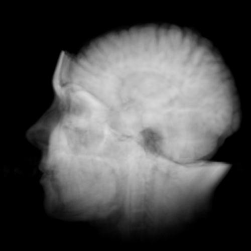
At a very high level of
description, you have an x-ray source, an image receptor (in the
old days a photographic plate), and something in between that
you want to look at. X-rays are partially blocked by dense
tissue like bones, and less blocked by soft tissue resulting in
an image on the image recepter where bones show up white and
softer tissue is darker. These are very portable (dentist
offices, emergency rooms) and very fast. The big disadvantage is
that a 3D volume like our chest or your tooth are compressed
into a 2D image which can make working out the 3D location
difficult.
More modern techniques create a sequence of slices that can be
combined to form a volume of data
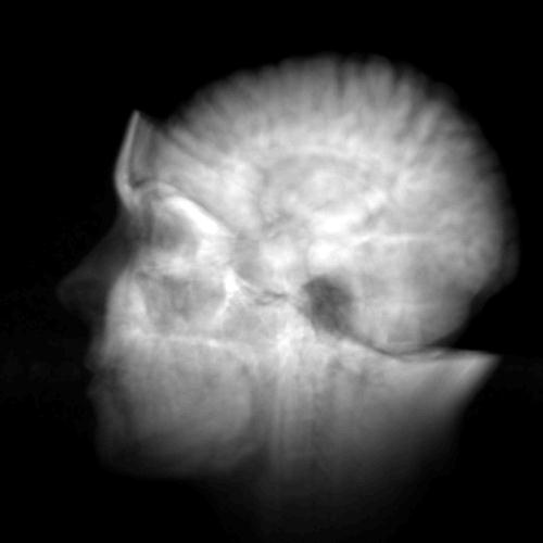
At a very high level of
description, a computed tomography scanner uses X-rays to take a
series of 2D images to combine into a 3D volume after a bunch of
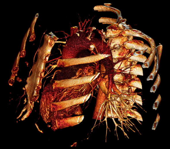
math is applied. CT scans are good for looking at bones. They
can also make use of contrast agents, typically iodine.
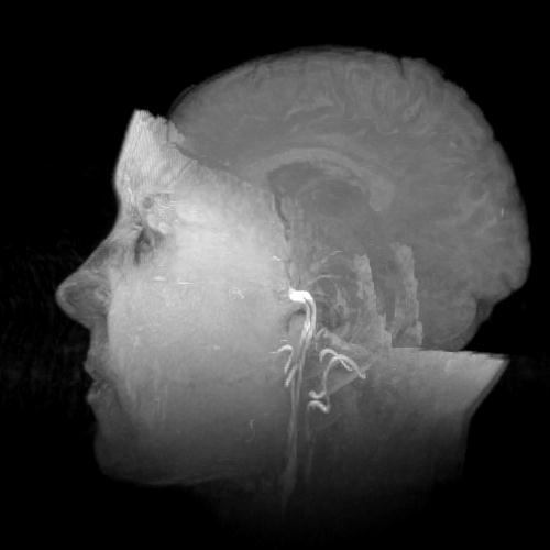
At a very high level of
description, Magnetic Resonance Imaging uses a powerful magnetic
field to align the hydrogen atoms in the water of the body with
the direction of the field. A radio frequency electromagnetic
field is introduced which causes the atoms to alter their
alignment. When the field is turned off they return to their
original alignment producing a detectable signal. Atoms in
different types of issue return to the original alignment at
different rates, based on the density of water in the tissue, so
a 3D picture of the different tissues can be built up through a
lot of math. If there isn't enough natural contrast between the
densities then a contrast agent can be introduced to
artificially boost the contrast. MRI
is good for looking at soft tissue and finding tumors.
CT typically has better
spatial resolution, but MRI has better contrast. MRI takes
longer (30 minutes for MRI vs 10 minutes for CT.) Note that
aside from a person needing to remain still during the scan,
organs like the heart and the lungs are not remaining still that
long. CT uses radiation which is bad. MRI uses strong magnetic
fields which may be bad. Both are constantly improving.
Functional Magnetic Resonance Imaging works like MRI
but the idea is to collect data in real-time (once every few
seconds), though at lower resolution, commonly from the brain.
From the virtual human web
page
(https://www.nlm.nih.gov/research/visible/visible_human.html)
"The Visible Human Male data set consists of MRI, CT and
anatomical images. Axial MRI images of the head and neck and
longitudinal sections of the rest of the body were obtained at 4
mm intervals. The MRI images are 256 pixel by 256 pixel
resolution. Each pixel having 12 bits of grey tone resolution.
The CT data consists of axial CT scans of the entire body taken
at 1 mm intervals at a resolution of 512 pixels by 512 pixels
with each pixel made up of 12 bits of grey tone. The
approximately 7.5 megabyte axial anatomical images are 2048
pixels by 1216 pixels, with each pixel defined by 24 bits of
color. The anatomical cross-sections are at 1 mm intervals to
coincide with the CT axial images. There are 1871 cross-sections
for both CT and anatomy. The complete male data set, 15
gigabytes in size, was made publicly available in November,
1994.
The Visible Human Female
data set, released in November, 1995, has the same
characteristics as the The Visible Human Male with one
exception, the axial anatomical images were obtained at 0.33 mm
intervals. This resulted in 5,189 anatomical images, and a data
set of about 40 gigabytes. Spacing in the "Z" direction was
reduced to 0.33mm in order to match the 0.33mm pixel sizing in
the "X-Y" plane, thus enabling developers interested in
three-dimensional reconstructions to work with cubic voxels."
(and let us remember that in
1995 personal computers were running at 200Mhz, with 16MB of RAM
and 1 GB hard drives. Now the visible woman dataset easily fits
on a USB stick)
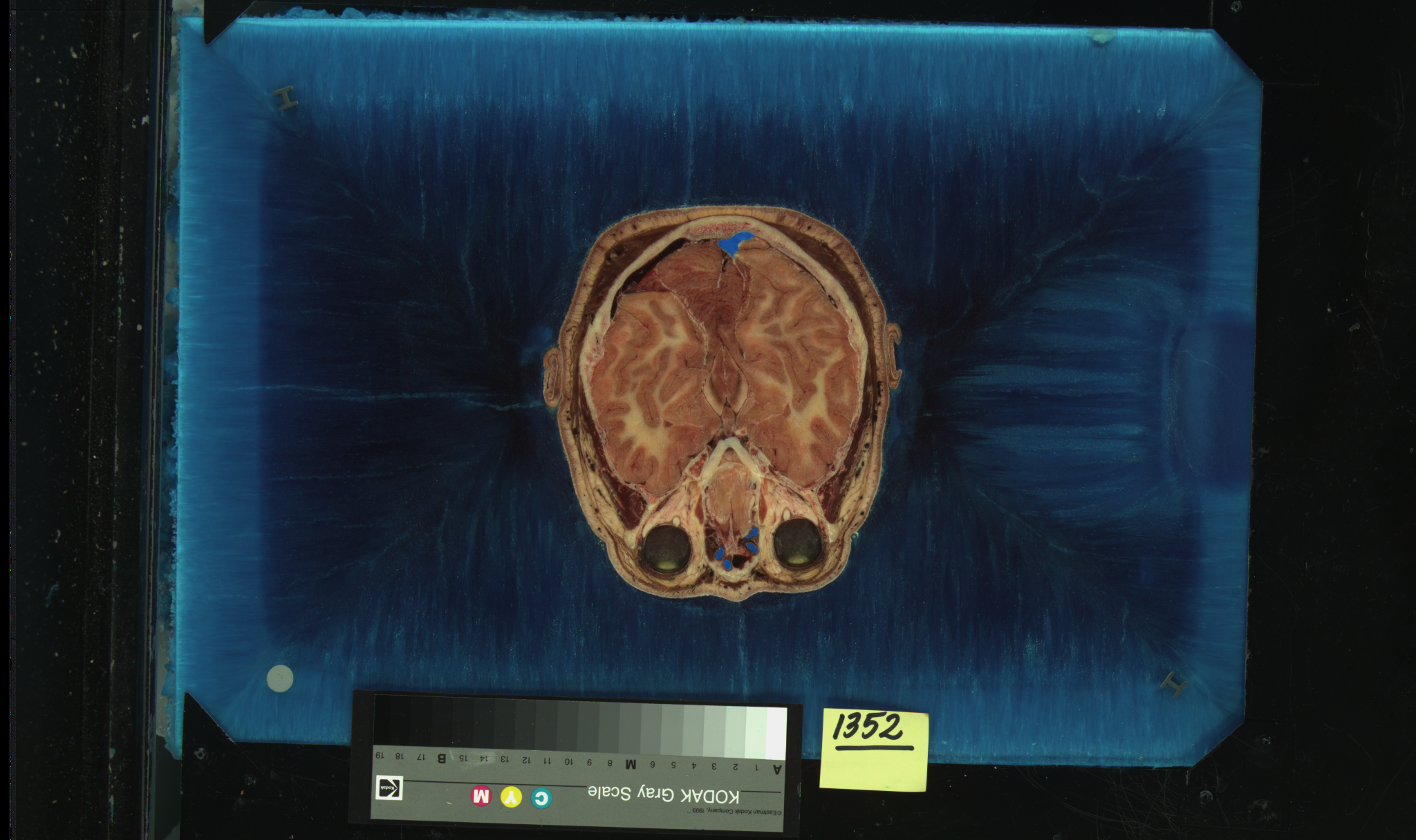
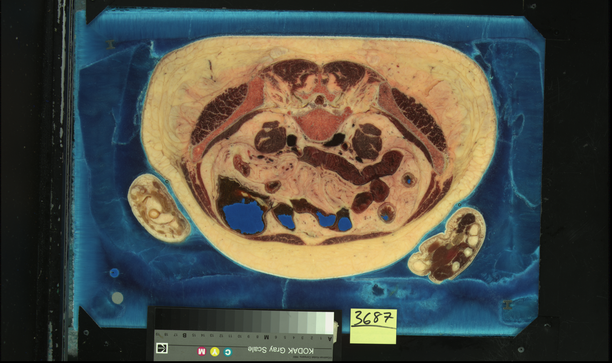
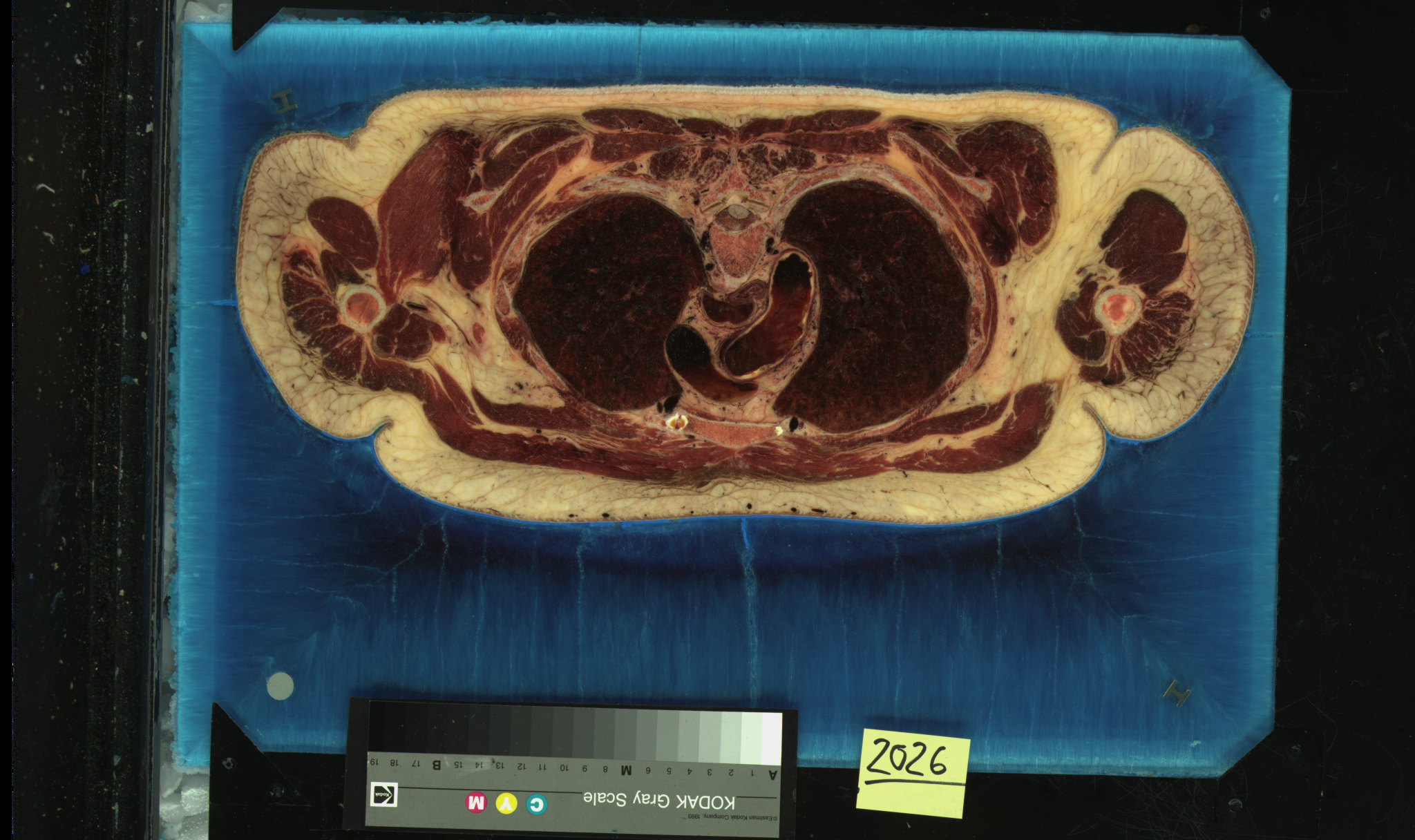
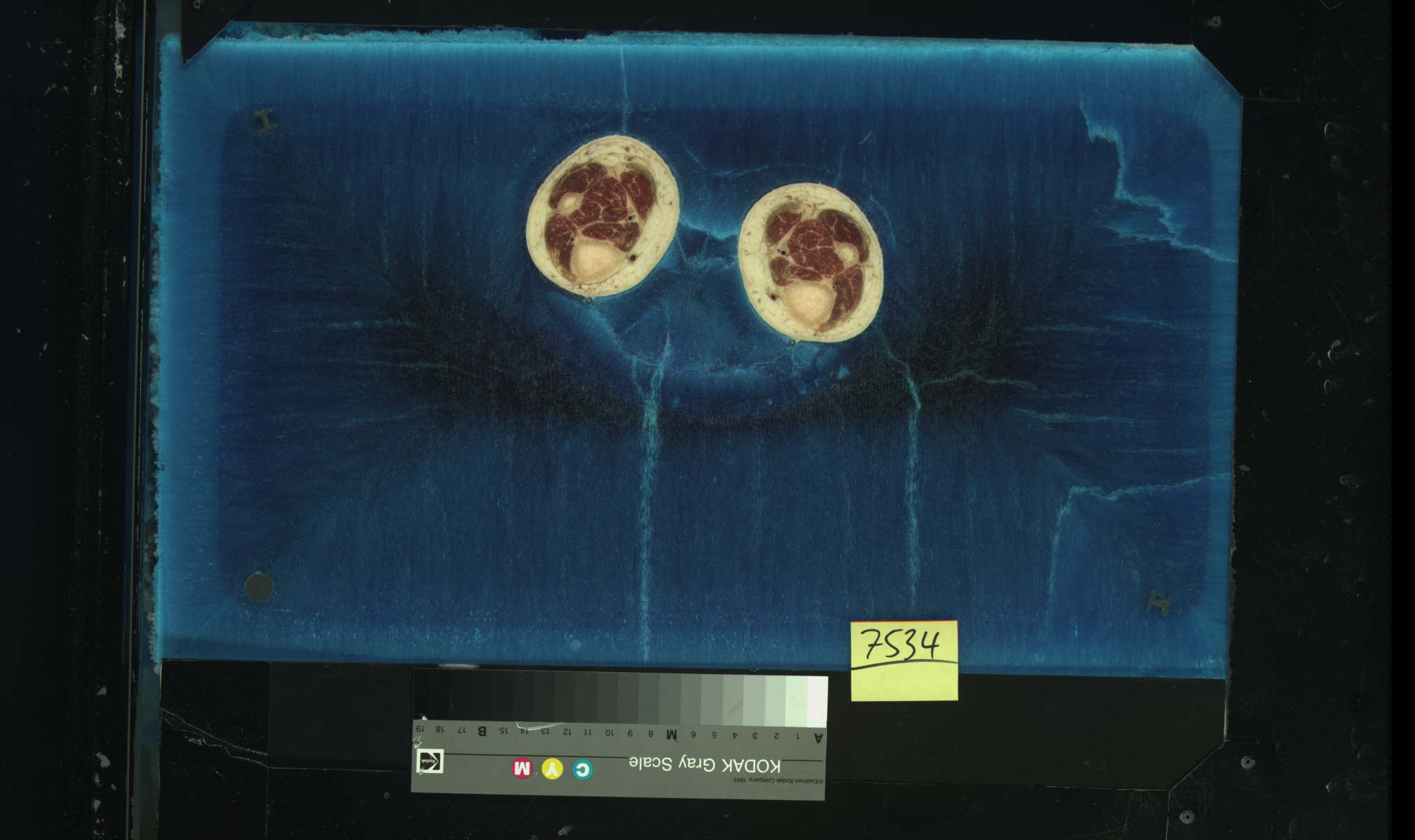
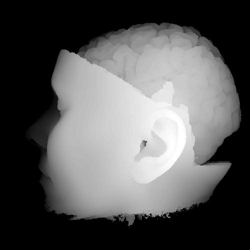
Here are some small JPEG
images of a very few of the slices of the visible woman. We will
show a movie in class of the full-size images. Once these images
were collected and aligned then images slicing through the body
on other planes are easy to generate as well as the ability to
generate arbitrary planes.
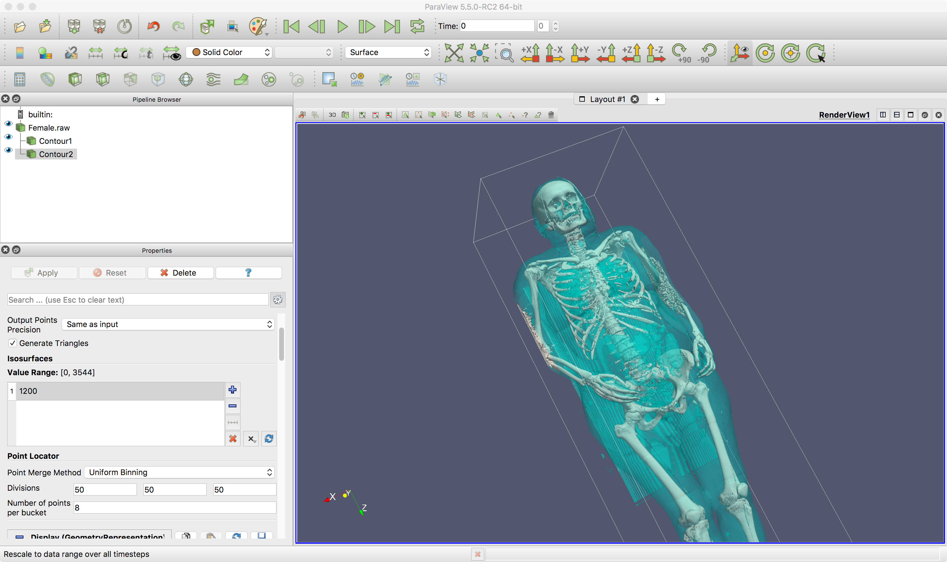
Here is ParaView viewing the
75MB version of the Visible Woman dataset. ParaView is a tool we
use in the graduate level scientific visualization course that
deals much more with 3D datasets. It is build on top of a
library called VTK (the visualization toolkit.) This allows us
to take the volumetric data and convert it into polygonal
surfaces.
This version of the dataset
is made up of 577 slices, 1 slice every 3mm, where each slice is
256 x 256 16-bit values. Note that this is not terribly high
resolution. Once the data is loaded in we can set up two
contours - one for the skin and one for the bones.
Since this is a 3d block of
data values we need to tell ParaView how to read in this data:
Data Scalar Type: unsigned short
Data Byte Order: BigEndian
File Dimensionality: 3
Data
Origin:
0 0 0
Data
Spacing: 1
1 1.33
Data
Extent:
0 255, 0 255, 0 576
Num Scalar Components: 1
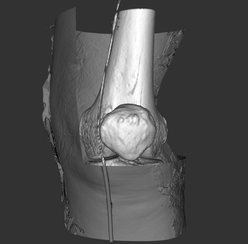
Once its read in I can then create 2 contours - one
transparent at 800 for skin, and one opaque at 1200 for bone to
create surfaces at those two boundaries. This results in
something similar to this.
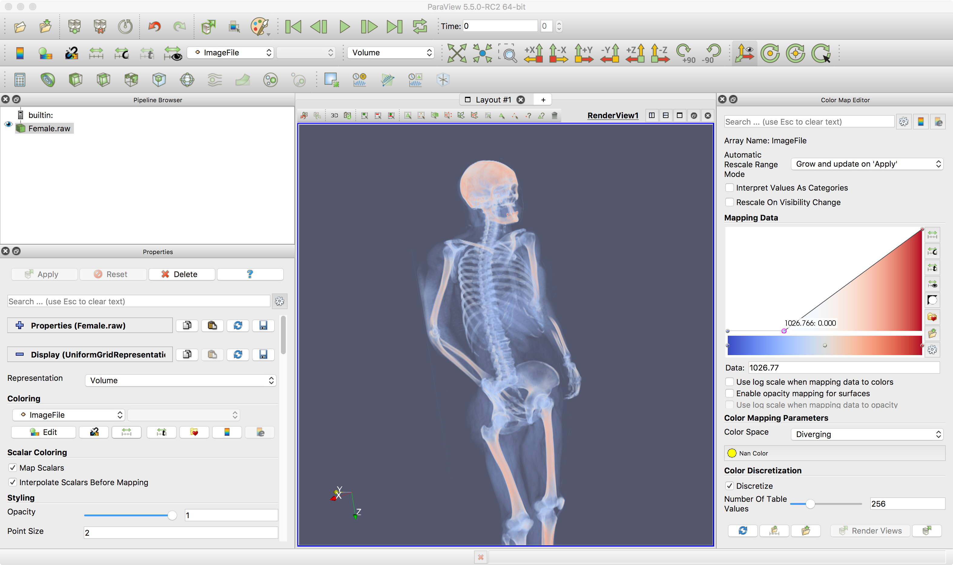
and another way is through volume rendering (change the
representation to volume) with the transfer function shown on the
right (right click edit color) where we assign colors and opacity
to different ranges of values in the block of data.
More recently newer scans have been made including
the Visible Korean Human and the Chinese Visible Human.
Paraview was designed to be
a general purpose tool so it is not particularly focused on
medical data - which makes it harder to use than the specialized
tools we will talk about later, but has the basic functionality
that students can recreate in the Computer Graphics II course.
Contouring - constructing
boundaries between regions
2D - contour lines of
constant scalar value
e.g. weather maps
annotated with lines of constant temperature
(isotherms)
e.g. topological maps
with lines of constant elevation
3D - isosurfaces - surfaces
of constant scalar value
e.g. skin or bone in a
medical image showing a constant intensity
generating contours probably
requires interpolation between the given points
generate a new set of points
then connect them into a contour
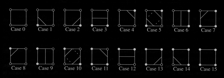
Marching Squares (2D) /
Marching Cubes (3D)
assumes a contour can
pass through a cell in only a finite number of ways
can create a table
enumerating all these possible topological states of
cell
# of states depends
on # of cell vertices and # of possible in/out
relationships
vertex is 'inside' if
scalar value > value of contour line
vertex is 'outside'
if scalar value < value of contour line
e.g. if cell has 4
vertices and each can be in or out then 16
possibilities
can
represent these by a 4 bit code
currently not
interested in 'where' the contour passes through
cell, just 'how'
treats each cell
independently
select cell
calculate inside/outside
for each vertex of the cell
create 4-bit index from
in/out values
use index to look up
topological state
interpolate contour
location for each edge
dark vertex is above the contour value (inside), white
vertex is below (outside)
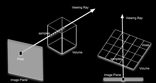
another way to look at this kind of data is
through Volume Rendering where we avoid generating polygons
a common way
is to use ray-casting
greyscale data values
minimum value = transparent
black
maximum value = white
determine values encountered
along ray
processing those values according
to ray function - many possibilities
volume is 3D image dataset w/
scalar values at points of a regular grid
need an interpolation function to
sample locations between the grid points
transfer function maps
information at voxel location into material / color / opacity
e.g. differentiating air,
muscle, bone in a CT scan
can have separate functions for
red, green, blue, opacity
Regions of Interest
often need to look through parts
of the volume to see other parts of the volume
can specify a partial region of
the volume to render that contains interesting things
use clipping planes or other
geometric forms to specify the region
Paraview is currently at version 5.10 and
you can download it from:
https://www.paraview.org/download/
There is a detailed introduction and
tutorial at:
https://www.paraview.org/Wiki/The_ParaView_Tutorial
and I'd like people to go through Chapter 2 Basic Usage through
2.8.
As usual you should start up a new Jupyter
notebook, take screenshots from ParaView as you progress
through the tutorial, and add those screen shots showing your
progress through each part. When you are done print to PDF and
upload it to Gradescope.
Scientific Visualization
In past terms we have had talks various by
people in this area that we have worked with:
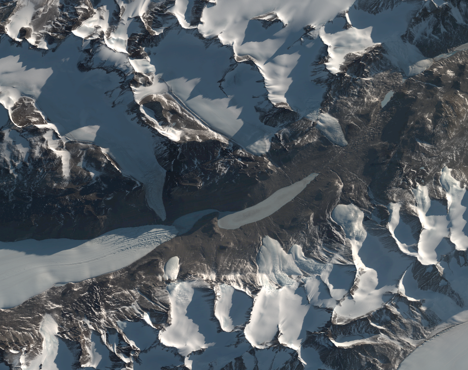
Paul Morin
Director of the Polar Geospatial Information Center
https://www.pgc.umn.edu/about/
Dr Mark SubbaRao
Astronomer
formerly at the Adler Planetarium
now leading NASA Goddard's Scientific Visualization Studio
Dr Peter Doran
Professor
Department of Geology and Geophysics
Louisiana State University
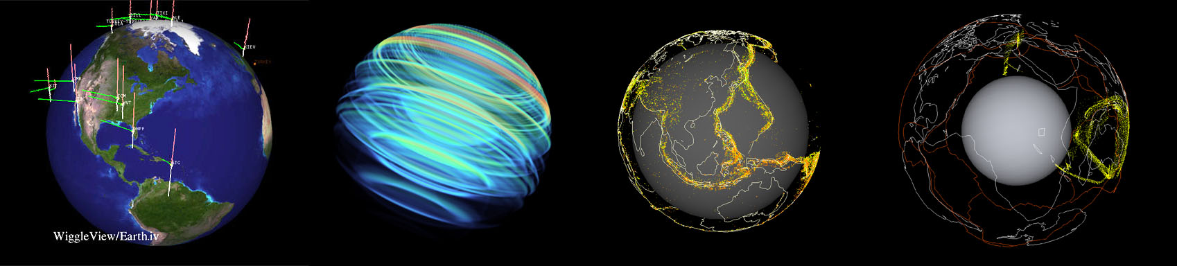
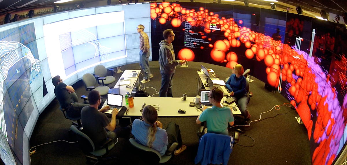
Three main uses for visualizing
scientific data
viewing / evaluating
collected data (is it complete, correct)
viewing / evaluating
simulation data (is
it complete, correct, should I stop and restart)
presenting data to a
different audience
Some fields like astronomy rely on
observation and simulation with very little chance for direct
experimentation, others like high energy physics have access to
very big experimental setups.
When doing analysis, you want to
be able to compare data collected at different times and places,
compare real data to simulated data, integrate data from
multiple real and simulated sources to solve more complex
problems.
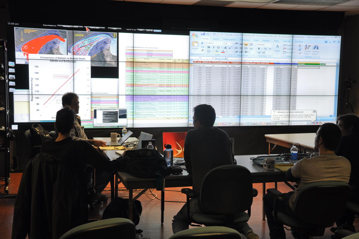
Here are a couple other specific use cases:
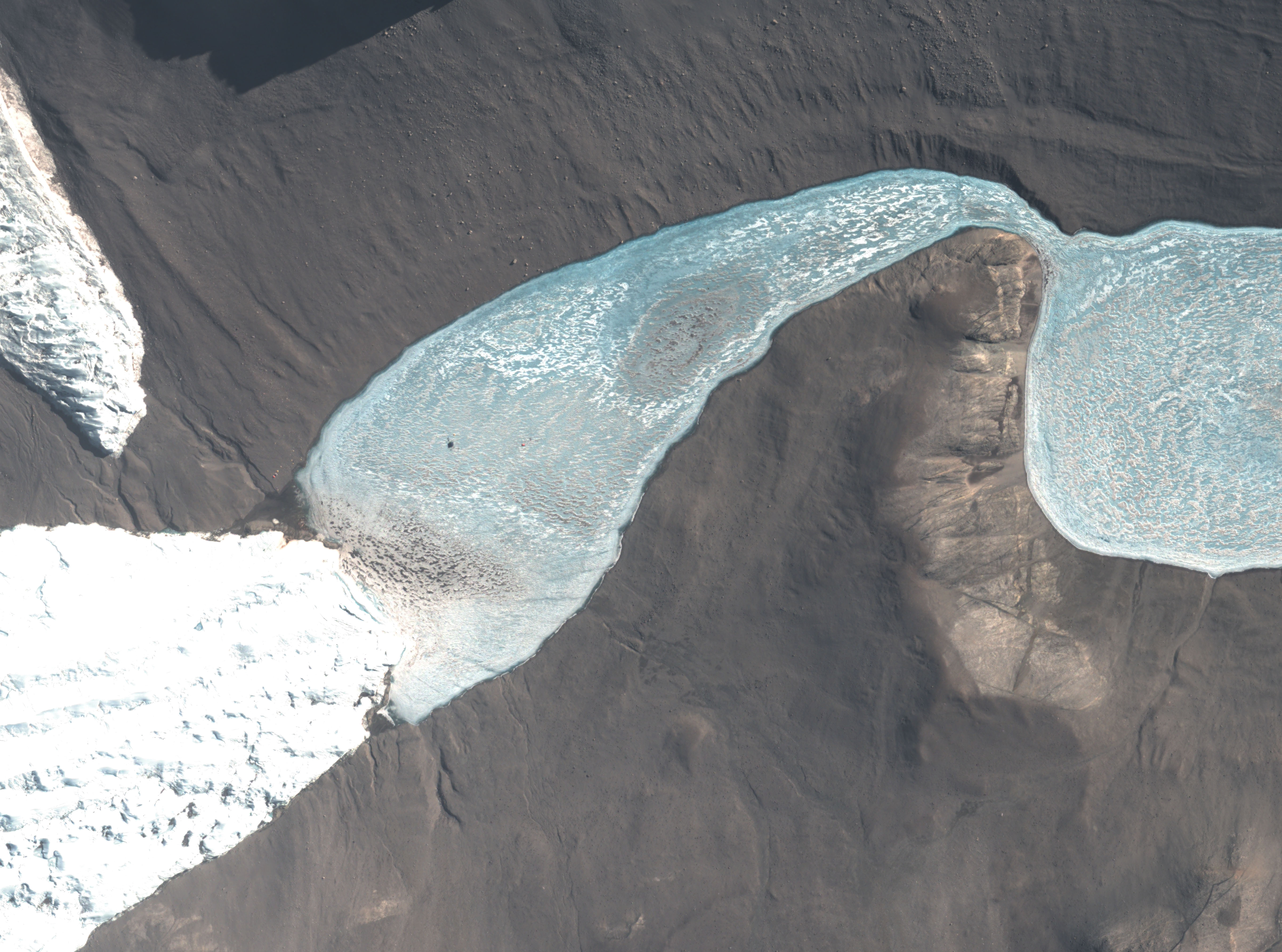
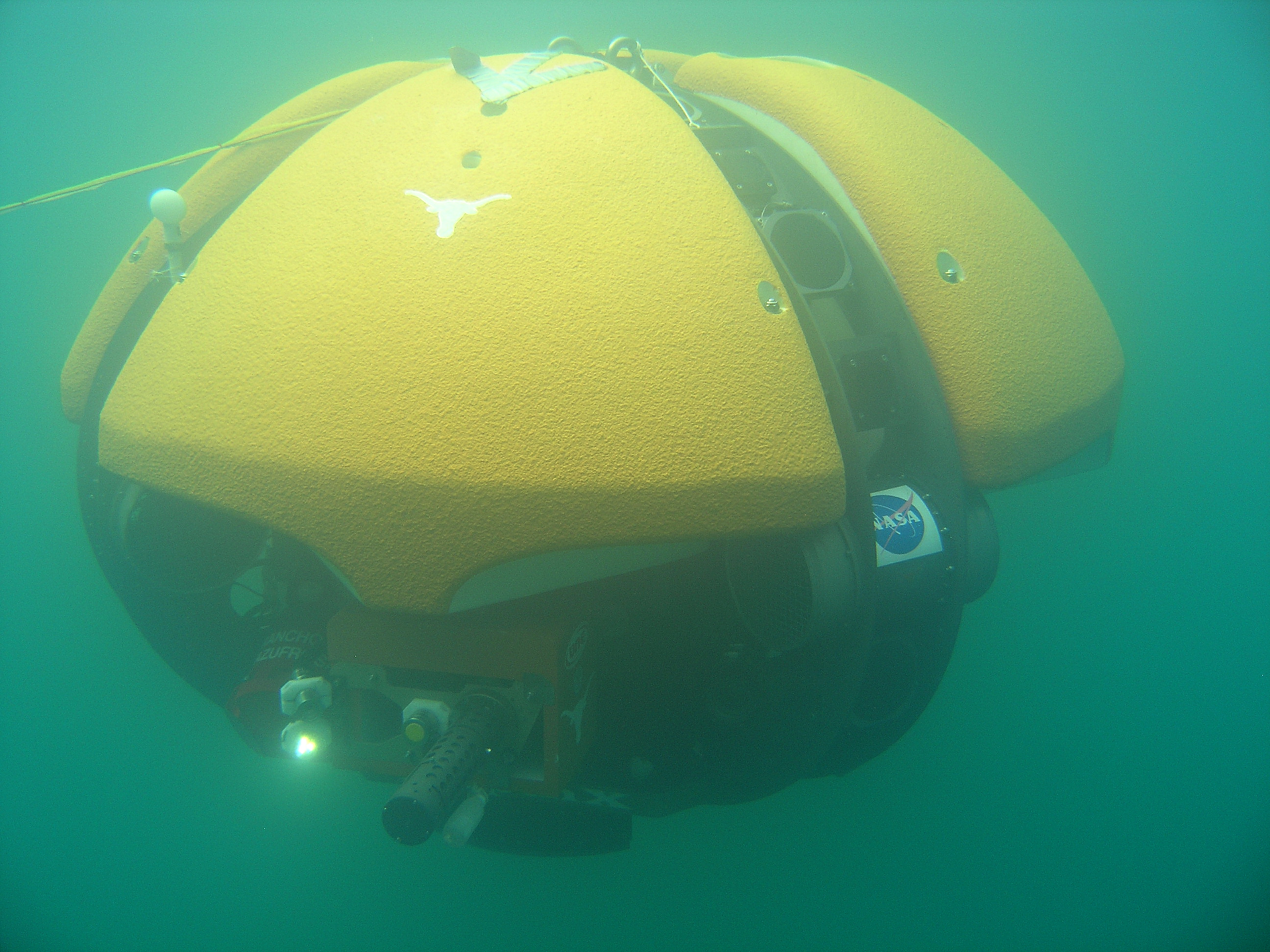
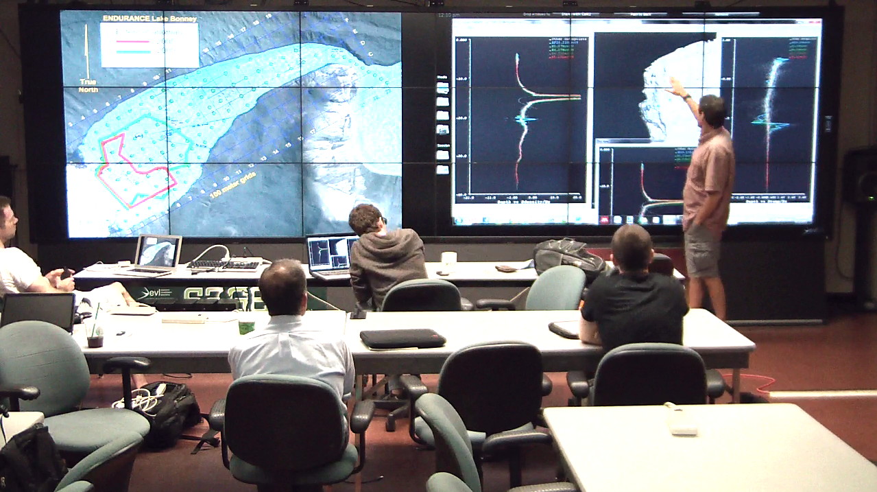
Endurance
have elevation of
the landscape around the lake
have older bathymetry data collected at various
points of the lake
have older chemistry data collected at various
points in the lake
Given that sparse data you can form hypotheses
and plan for more thorough data collection
Goals:
generate accurate bathymetry for
the lake
investigate the chemical
composition of the entire volume of the lake
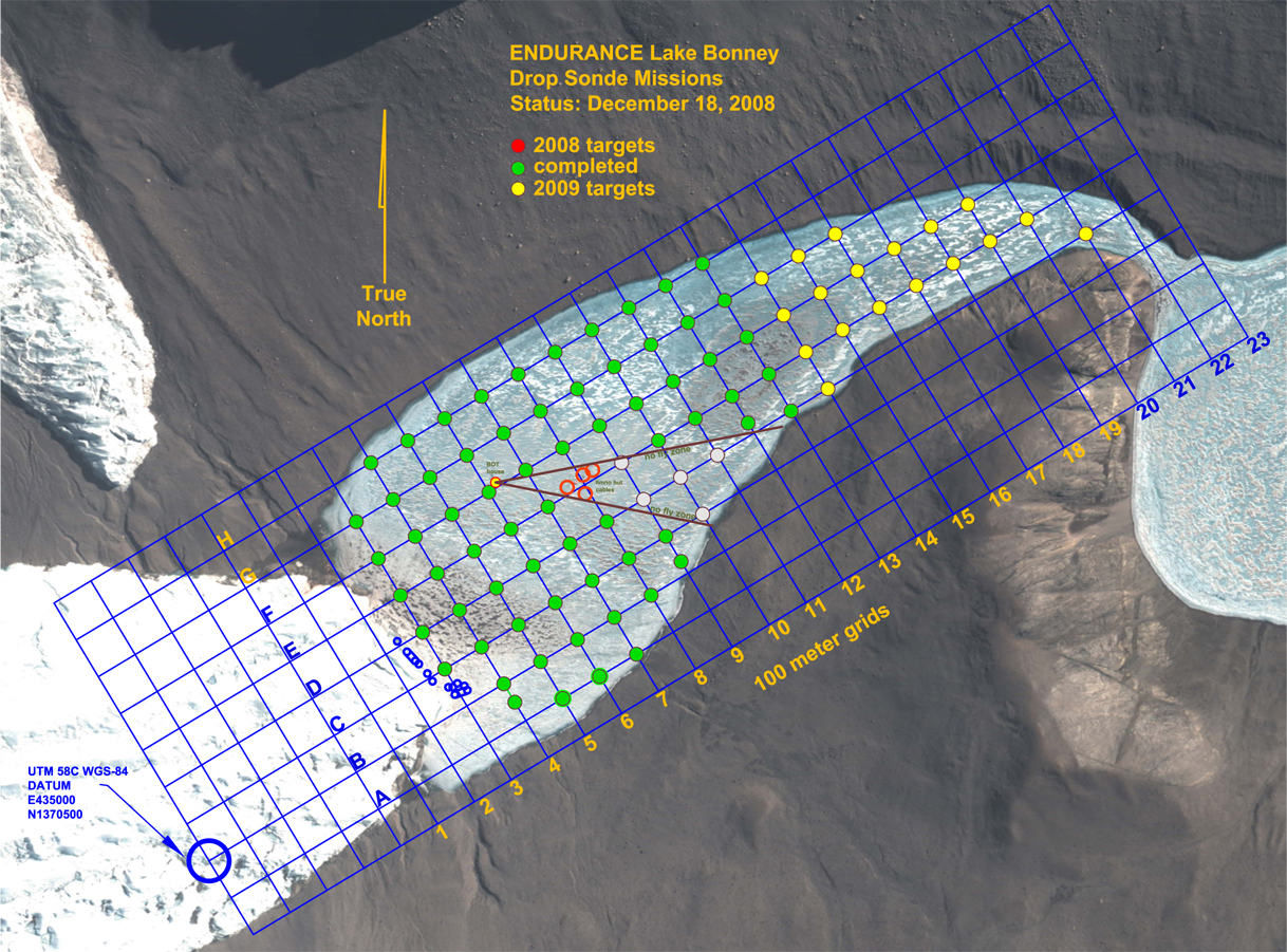
Mission in December 2008
Mission in November 2009
collecting current multispectral satellite
photography at beginning and end of deployment
collecting GPS readings at various locations on
site to correctly map the satellite photography to the terrain
collecting information on lake level each day
collecting data on new bathymetry directly on a 100m by 100m 2D grid collecting
data on new bathymetry via constant sonar
collecting data on chemical content of the lake
on a 100m by 100m by every-few-centimeters 3D grid
Conductivity (S/m)
Temperature (C )
CDOM (ru)
Chl-a (ru)
REDOX (meV)
PAR (umol/m^2*s^1)
pH
Turbidity (ru)
collecting
photographs of the ice from below on a 100m by 100m 2D grid
each day there is one mission where the vehicle
starts from the same site and goes off to several of the
measurement sites and collects data.
however
the water level in the
lake changes from day to day and year to year meaning 'depth'
is relative
there is a layer of high
salinity in the lake which disrupts the sonar
a stream starts flowing in
the middle of data collection changing the chemical makeup of
the lake
instruments don't always
work properly
first
make a copy of the
collected data each day as a backup
look at collected data -
in particular the n files of CSV numerical data
do the numbers make
sense? excel or some other simple graphing tool is your
friend
check min, max, general
trends, odd outliers, dramatic changes in value
what if some of the
measurements are clearly wrong? if a device failed when did it
fail and how many measurements are affected? instead of
looking at missions independently you now need to look at them
in temporal order
ideally you do all of this in the field so you
know if you missed collecting any data so you run another mission
and collect it again.
next
need to assign common null
values to make later processing easier (might be tricky with
different types of data)
need to correct depth
issues (where is depth gauge on the vehicle, what is current
lake level - this affects the precise depth of all the
measurements
need to keep track of the
changes being made to the data - a copy (and backup) of the
raw data should remain untouched. Revised versions of the data
should have metadata describing the changes that were made.
need to explicitly state
what is the degree of accuracy of each instrument
now we can get to more interesting
visualization and analysis issues
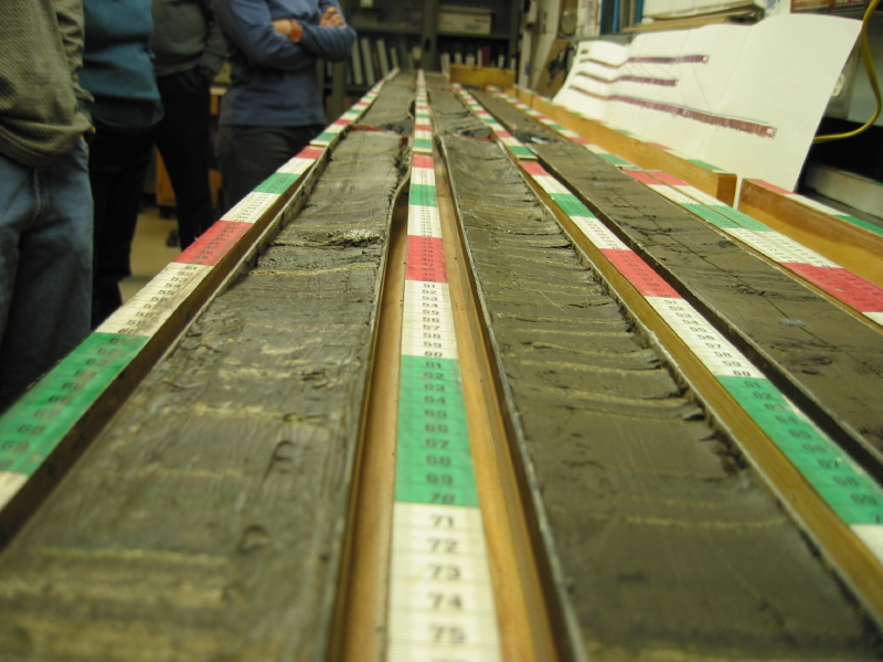
CoreWall
Cores brought up from lakes,
ice, ocean floor, the antarctic These cores may be several
meters long or several kilometers long
Used to determine the climate
thousands to hundreds of millions of years ago
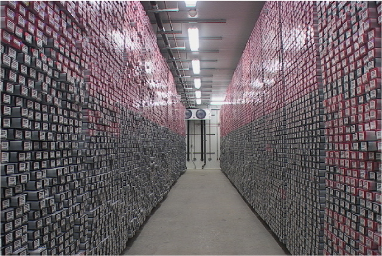
Cores brought up and sliced in
half
One half kept untouched in
refrigerated storage
One half is photographed
and sampled and then put into refrigerated storage
Data from each core segment is
recorded on a paper 'barrel sheet' summary stored in binders
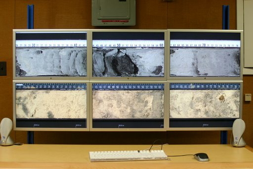
printouts of the
photographic scan of the core
graphs of measurements
taken along the core
information on samples
collected from specific points of the core
Why doesn't this work
Researchers must go to the
core to collect new tests
Researchers may have to
wait months before physical cores are shipped back from drill
site
Cores in storage oxidize,
shrink
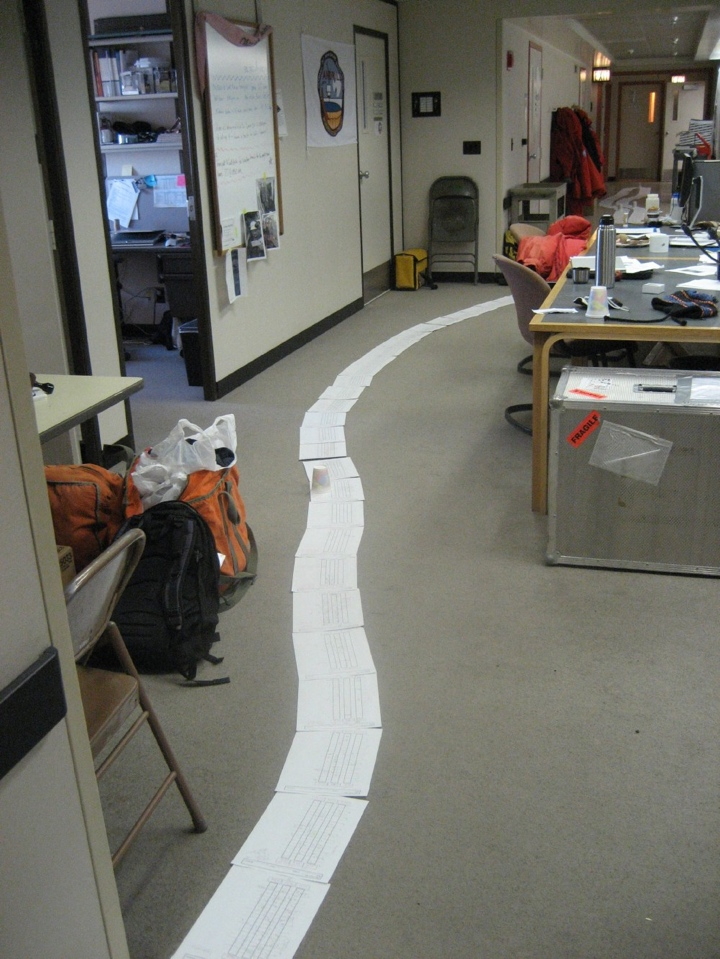
Paper in binders is not an
easily sharable format
to look at long cores
investigators need to lay paper end to end down the hallway
cores can be scanned at
higher resolution than eventual data storage - that
information is wasted
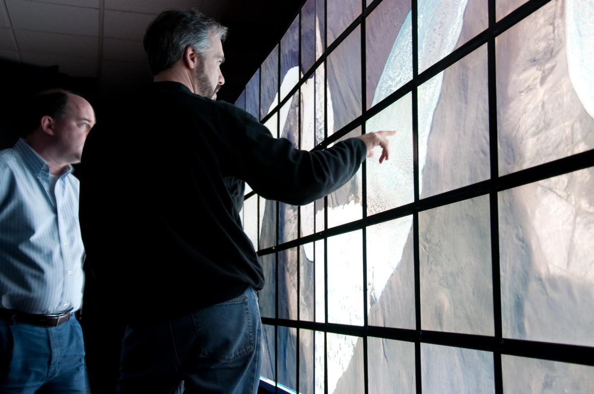
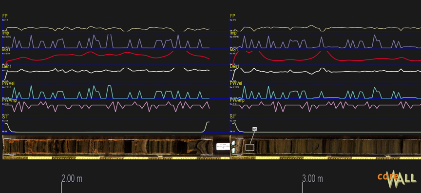
CoreWall solution
keep information in
digital form (photography, numerical scans, annotations)
store data in common
database(s) allowing remote access over the internet
information immediately
available when it is scanned at the drill site
use multiple high
resolution monitors to allow people to load in multiple core
segments, pan, and zoom, in the lab
easy to find and compare
related core data (from previous expeditions, from nearby
drill sites)
same software runs on a
laptop for personal work
ANDRILL 2006 - two
CoreWall setups in Antarctica
ANDRILL 2007 - seven CoreWall setups including one at the drill
site in Antarctica
now installed on JOIDES Resolution drill ship