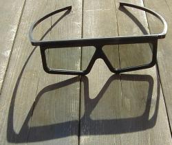
People like wearing
sunglasses - lightweight, stylish, useful
People are used to wearing passive glasses at the theatre
to see 3D movies - lightweight, useful
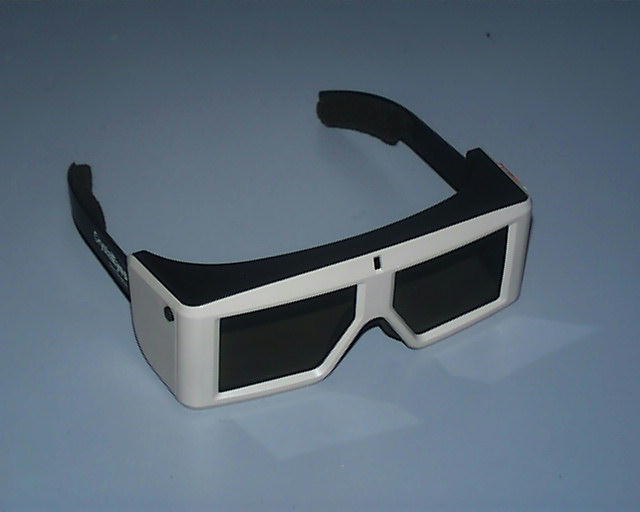
People do not like wearing heavy or unbalanced glasses
People do not like wearing helmets
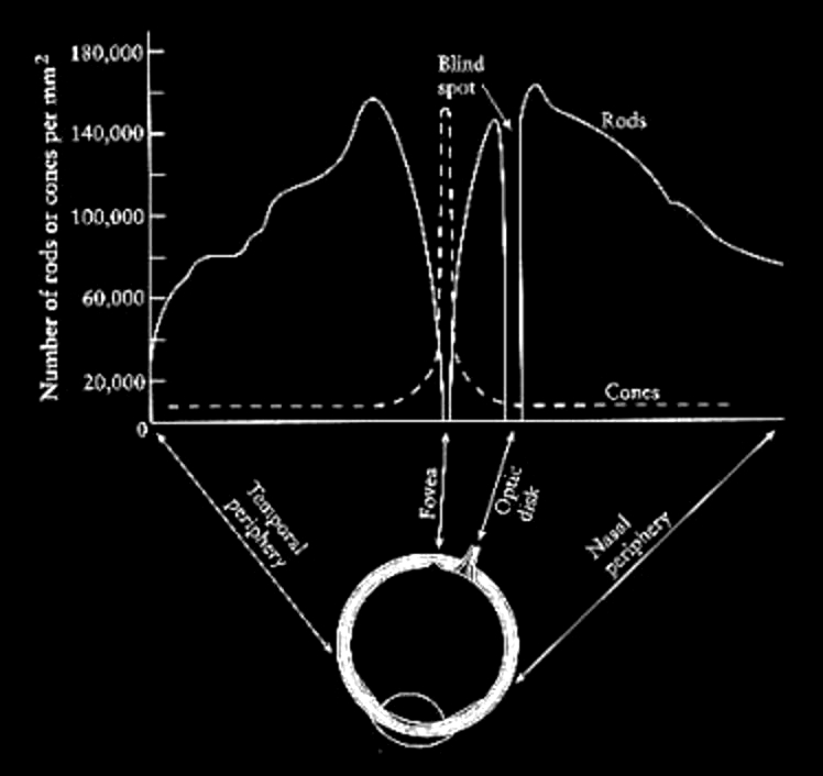
Human eye has 2 types of photosensitive receptors: cones and
rods
cones
operate at higher
illumination levels
provide better
spacial resolution and contrast sensitivity
provide colour
vision
rods
operate at lower
illumination levels, most sensitive to green
The
cones are highly concentrated at the fovea and quickly taper off
around the retina. For colour vision we have the greatest acuity
at the fovea, or approximately at the center of out field of
vision. Visual acuity drops off as we move away from the center
of the field of view. However, we are very sensitive to motion
on the periphery of our vision, so we can see movement even if
we can't see what is moving.
The rods are highly
concentrated 10-20 degrees around the fovea, but almost none are
at the fovea itself - which is why if you are stargazing and
want to see something dim you can not look directly at it.
There is also the optic
nerve which is 10-20 degrees away from the fovea which connects
your eye to your brain. This is the blind spot where there are
no cones and no rods. We can not see anything at this point
though we are so used to this that we do not notice it unless we
try to see the blind spot.
The eye has a dynamic range of 7 orders of magnitude
Eye is sensitive to ratios of intensities not absolute magnitude.
Brightness = Luminance^0.33. To make something appear n times
brighter the luminance must be increased by n^3.
Colour
Most perceptual processes are driven by intensity not colour.
Motion system is colour blind, depth perception is colour blind,
object recognition is colour blind.
but uniquely coloured objects are easy to find
8 percent of men are color blind
1 percent of women are color blind
Are you colour blind? You can check on Wikipedia -
http://en.wikipedia.org/wiki/Ishihara_color_test
Each eye has approximately 150 degrees horizontal (60 degrees
towards the nose and 90 degrees to the side) and 120 degrees
vertically (50 degrees up and 80 degrees down)
Below is an 'eye chart' showing the resolutions of various VR
devices from the early 1990s when the CAVE was introduced. From
left to right: 20/20 (6/6 in the metric world), CRT 20/40, HMD
20/425, BOOM 20/85, and CAVE 20/110 using the Snellen fraction
(20/X where this viewer sees at 20 feet detail that the average
person can see at x feet, 20/200 is legally blind)
Temporal Resolution
The real world doesn't flicker (aside from things like florescent
lights). Some people can perceive flickering even at 60Hz (the
image being refreshed 60 times per second) for a bright display
with a large field of view but most people stop perceiving the
flicker between 15Hz (for dark images) and 50Hz (for bright
images).
Convergence and Accommodation for 3D scenes
In a 3D display
environment the brain is getting two different cues about the
virtual world. Some of these cues indicate this world is 3D
(convergence and stereopsis). Some of these cues indicate that the
world is flat (accomodation).
The eyes are focusing on the screen but they are converging
depending on the position of the virtual objects which could be in
front of, on, or behind the screen
Note that only 90-95% of the population can see in stereo
Simulator sickness
2 things are needed: a functioning vestibular system (canals in
the inner ear) and a sense of motion
These symptoms can persist after the experience is finished.
Causes: still unknown but one common hypothesis is a mismatch
between visual motion (what your eyes tell you) and the vestibular
system (what your ears tell you)
Why would this cause us to become sick? Possibly an inherited
trait - a mismatch between the eyes and ears might be caused by
ingesting a poisonous substance so vomiting would be helpful in
that case.
sense of motion is required
bright images are more likely to cause it than dark ones
wide field of view is more likely to cause it than narrow field of
view
low resolution, low frame rate and high latency are also likely
causes
Another hypothesis deals with the lack of a rest frame. When a
user views images on a screen with an obvious border that border
locates the user in the real world. Without that border the user
loses his/her link to the real world and the affects of motion in
the virtual world are more pronounced.
fighter pilots have 20 to 40 percent sickness rates in flight
simulators - but experienced pilots get sick more often than
novice pilots.
In a rotating field when walking forward, people tilt their heads
and feel like they are rotating in the opposite direction.
This all affects the kinds of imagery you display and how it can
move. Open fields are less likely to cause problems than walking
through tight tunnels; tunnels are very aggressive in terms
of peripheral motion. This doesn't mean you should have any
tunnels, but you should be careful how much time the users spend
there.
For Thursday's Class
If your UIN ends in an
odd number you should read this paper and produce a similar 1 page
report to show on the wall and perhaps discuss.
Sizing up visualizations: effects
of display size in focus+ context, overview+ detail, and
zooming interfaces
Jakobsen, Hornbaek
Proceedings of the SIGCHI Conference on Human Factors in
Computing Systems 2011 http://dl.acm.org/citation.cfm?id=1979156
If your UIN ends in an even number you should read this paper and produce a similar 1 page report to show on the
wall and perhaps discuss.
Beyond visual acuity: the perceptual
scalability of information visualizations for large
displays
Yost, Haciahmetoglu, North
Proceedings of the SIGCHI Conference on Human
Factors in Computing Systems 2007 http://dl.acm.org/citation.cfm?id=1240639
Again, you should produce a 1 page critique
of the paper to put up on the wall Tuesday in class, and a subset of the students will
be asked to talk more in depth about the paper.