So far in the class we have dealt with simple wireframe drawings of the models. The main reason for this is so that we did not have to deal with hidden surface removal. Now we want to deal with more sophisticated images so we need to deal with which parts of the model obscure other parts of the model.
online, you can click here to see some images created by members of the Electronic Visualization Laboratory here at UIC. Each lecture has a different set of images (collect em all!)
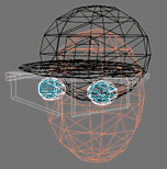
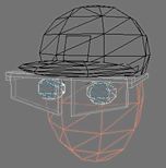
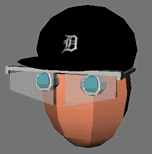
The following sets of images show a wireframe version, a wireframe version with hidden line removal, and a solid polygonal representation of the same object.
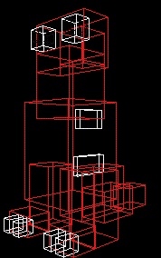
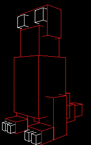
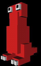
If we do not have a way of determining which surfaces are visible then which surfaces are visible depends on the order in which they are drawn with surfaces being drawn later appearing in front of surfaces drawn previously as shown below:
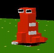
Here the fins on the back are visible because they are drawn after the body, the shadow is drawn on top of the monster because it is drawn last. Both legs are visible and the eyes just look really weird.
We do not want to draw surfaces that are hidden. If we can quickly compute which surfaces are hidden, we can bypass them and draw only the surfaces that are visible.
We also want to avoid having to draw the polygons in a particular order. We would like to tell the graphics routines to draw all the polygons in whatever order we choose and let the graphics routines determine which polygons are in front of which other polygons.
The idea is to speed up the drawing, and give the programmer an easier time, by doing some computation before drawing.
Unfortunately these computations can take a lot of time, so special purpose hardware is often used to speed up the process.
Two types of approaches:
object space algorithms do their work on the objects themselves before they are converted to pixels in the frame buffer. The resolution of the display device is irrelevant here as this calculation is done at the mathematical level of the objects
for each object a in the scene
    determine which parts of object a are visible
    (involves comparing the polyons in object a to other polygons in a
    and to polygons in every other object in the scene)
image space algorithms do their work as the objects are being converted to pixels in the frame buffer. The resolution of the display device is important here as this is done on a pixel by pixel basis.
for each pixel in the frame buffer
    determine which polygon is closest to the viewer at that pixel location
    colour the pixel with the colour of that polygon at that location
As in our discussion of vector vs raster graphics earlier in the term the mathematical (object space) algorithms tended to be used with the vector hardware whereas the pixel based (image space) algorithms tended to be used with the raster hardware.
When we talked about 3D transformations we reached a point near the end when we converted the 3D (or 4D with homogeneous coordinates) to 2D by ignoring the Z values. Now we will use those Z values to determine which parts of which polygons (or lines) are in front of which parts of other polygons.
There are different levels of checking that can be done.
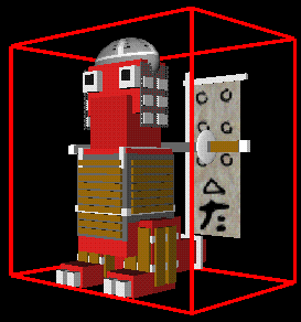
There are also times when we may not want to cull out polygons that are behind other polygons. If the frontmost polygon is transparent then we want to be able to 'see through' it to the polygons that are behind it as shown below:
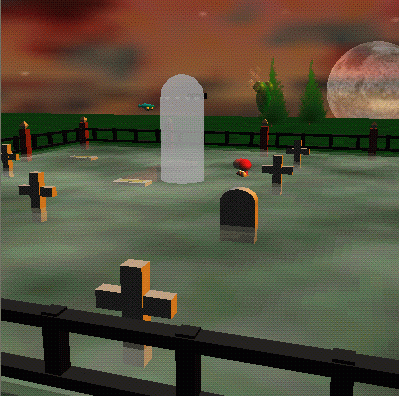
Which objects are transparent in the above scene?
We used the idea of coherence before in our line drawing algorithm. We want to exploit 'local similarity' to reduce the amount of computation needed (this is how compression algorithms work.)
Rather than dealing with a complex object, it is often easier to deal with a simpler version of the object.
in
2: a bounding box
in 3d: a bounding volume (though we still call it a bounding box)
We convert a complex object into a simpler outline, generally in the shape of a box and then we can work with the boxes. Every part of the object is guaranteed to fall within the bounding box.
Checks can then be made on the bounding box to make quick decisions (ie does a ray pass through the box.) For more detail, checks would then be made on the object in the box.
There are many ways to define the bounding box. The simplest way is to take the minimum and maximum X, Y, and Z values to create a box. You can also have bounding boxes that rotate with the object, bounding spheres, bounding cylinders, etc.
Back-face culling (an object space algorithm) works on 'solid' objects which you are looking at from the outside. That is, the polygons of the surface of the object completely enclose the object.
Every planar polygon has a surface normal, that is, a vector that is normal to the surface of the polygon. Actually every planar polygon has two normals.
Given that this polygon is part of a 'solid' object we are interested in the normal that points OUT, rather than the normal that points in.
OpenGL specifies that all polygons be drawn such that the vertices are given in counterclockwise order as you look at the visible side of polygon in order to generate the 'correct' normal.
Any polygons whose normal points away from the viewer is a 'back-facing' polygon and does not need to be further investigated.
To find back facing polygons the dot product of the surface normal of each polygon is taken with a vector from the center of projection to any point on the polygon.
The dot product is then used to determine what direction the polygon is facing:
Back-face culling can very quickly remove unnecessary polygons. Unfortunately there are often times when back-face culling can not be used. For example if you wish to make an open-topped box - the inside and the ouside of the box both need to be visible, so either two sets of polygons must be generated, one set facing out and another facing in, or back-face culling must be turned off to draw that object.
in OpenGL back-face culling is turned on using:
    glCullFace(GL_BACK);
    glEnable(GL_CULL_FACE);
Early on we talked about the frame buffer which holds the colour for each pixel to be displayed. This buffer could contain a variable number of bytes for each pixel depending on whether it was a greyscale, RGB, or colour-indexed frame buffer. All of the elements of the frame buffer are initially set to be the background colour. As lines and polygons are drawn the colour is set to be the colour of the line or polygon at that point. T
We now introduce another buffer which is the same size as the frame buffer but contains depth information instead of colour information.
z-buffering (an image-space algorithm) is another buffer which maintains the depth for each pixel. All of the elements of the z-buffer are initially set to be 'very far away.' Whenever a pixel colour is to be changed the depth of this new colour is compared to the current depth in the z-buffer. If this colour is 'closer' than the previous colour the pixel is given the new colour, and the z-buffer entry for that pixrl is updated as well. Otherwise the pixel retains the old colour, and the z-buffer retains its old value.
Here is a pseudo-code algorithm
for each polygon
    for each pixel p in the polygon's projection
	{
	pz = polygon's normalized z-value at (x, y); //z ranges from -1 to 0
	if (pz > zBuffer[x, y]) // closer to the camera
	    {
	    zBuffer[x, y] = pz;
	    framebuffer[x, y] = colour of pixel p
	    }
	}
This is very nice since the order of drawing polygons does not matter, the algorithm will always display the colour of the closest point.
The biggest problem with the z-buffer is its finite precision, which is why it is important to set the near and far clipping planes to be as close together as possible to increase the resolution of the z-buffer within that range. Otherwise even though one polygon may mathematically be 'in front' of another that difference may disappear due to roundoff error.
These days with memory getting cheaper it is easy to implement a software z-buffer and hardware z-buffering is becoming more common.
In OpenGL the z-buffer and frame buffer are cleared using:
glClear(GL_DEPTH_BUFFER_BIT | GL_COLOR_BUFFER_BIT);
In OpenGL z-buffering is turned on using:
glEnable(GL_DEPTH_TEST);
The depth-buffer is especially useful when it is difficult to order the polygons in the scene based on their depth, such as in the case shown below:

Warnock's algorithm is a recursive area-subdivision algorithm. Warnock's algorithm looks at an area of the image. If is is easy to determine which polygons are visible in the area they are drawn, else the area is subdivided into smaller parts and the algorithm recurses. Eventually an area will be represented by a single non-intersecting polygon.
At each iteration the area of interest is subdivided into four equal areas. Each polygon is compared to each area and is put into one of four bins:
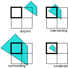
For a given area:
1. If all polygons are disjoint then the background colour fills the area
2. If there is a single contained polygon or intersecting polygon then the background colour is used to fill the area, then the part of the polygon contained in the area is filled with the colour of that polygon
3. If there is a single surrounding polygon and no intersecting or contained polygons then the area is filled with the colour of the surrounding polygon
4. If there is a surrounding polygon in front of any other surrounding, intersecting, or contained polygons then the area is filled with the colour of the front surrounding polygon
Otherwise break the area into 4 equal parts and recurse.
At worst log base 2 of the max(screen width, screen height) recursive steps will be needed. At that point the area being looked at is only a single pixel which can't be divided further. At that point the distance to each polygon intersecting,contained in, or surrounding the area is computed at the center of the polygon to determine the closest polygon and its colour,
Below
is an example scanned out of the text:
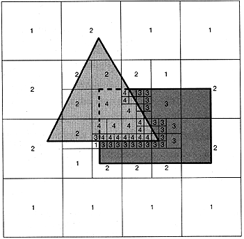
Here is a place where the use of bounding boxes can speed up the process. Given that the bounding box is always at least as large as the polygon, or object checks for contained and disjoint polygons can be made using the bounding boxes, while checks for interstecting and surrounding can not.
More Visible-Surface Determination