Week 4

Fancier Stuff

Simple Animation

Need to pass some time-code or counter into the shader from the OpenGL application.

One example is blending two texture maps based on a counter.

vertex shader:

varying vec2 TexCoord;

void main (void)
{
    TexCoord = gl_MultiTexCoord0;
    gl_Position = ftransform();

}

fragment shader:

uniform sampler2D tex;
uniform sampler2D tex2;

uniform float Alpha;

varying vec2 TexCoord;

void main(void)
{
    float A = max(sin(Alpha), 0.0);
    vec3 textureColor = vec3(texture2D(tex, TexCoord.st));
    vec3 textureColor2 = vec3(texture2D(tex2, TexCoord.st));

    vec3 color = textureColor * A + textureColor2 * (1.0 - A);
    gl_FragColor = vec4 (color, 1.0);
}

and in openGL:

    glActiveTexture(GL_TEXTURE0);
    glBindTexture(GL_TEXTURE_2D, texNumOn);

    glActiveTexture(GL_TEXTURE1);
    glBindTexture(GL_TEXTURE_2D, texNumOff);

    static float blender = 0.0;

    tex0Loc = glGetUniformLocation(p, "tex0");
    glUniform1i(tex0Loc, 0); // should match GL_TEXTURE0 above

    tex1Loc = glGetUniformLocation(p, "tex1");
    glUniform1i(tex1Loc, 1); // should match GL_TEXTURE1 above


    alphaLoc = glGetUniformLocation(p, "Alpha");
    glUniform1f(alphaLoc, blender);

    blender += 0.001;

where previously the textures were bound when they were loaded to 0 (texNumOn) and 1 (texNumOff)

To create a cycle between these two images:
off version of the
sign

Remember that you can't send a GL texture ID (which is a GLuint that is usually generated by glGenTextures) as your sampler, so you cant ask OpenGL for a textureID and then pass that along. The GL texture ID is only valid in the main program. A sampler should be from 0 to the maximum number of texture image units.

Code is available for the application, the vertex shader, and the fragment shader.

Another example is a wobble as described in chapter 16 of the Orange Book (chapter 13 of the first edition) where a sin function is used to perturb the texture coordinates. In the Orange book the sin is apprximated since the sin function didnt exist in GLSL at that point in time.

wobbling texture

Vertex Shader

// Vertex shader for wobbling a texture
// Author: Antonio Tejada
// Copyright (c) 2002-2004 3Dlabs Inc. Ltd.
// See 3Dlabs-License.txt for license information

varying float LightIntensity;
uniform vec3 LightPosition;

varying vec2 TexCoord;

const float specularContribution = 0.1;
const float diffuseContribution = 1.0 - specularContribution;

void main(void)
{
    vec3 ecPosition = vec3 (gl_ModelViewMatrix * gl_Vertex);
    vec3 tnorm      = normalize(gl_NormalMatrix * gl_Normal);
    vec3 lightVec   = normalize(LightPosition - ecPosition);
    vec3 reflectVec = reflect(-lightVec, tnorm);
    vec3 viewVec    = normalize(-ecPosition);

    float spec      = clamp(dot(reflectVec, viewVec), 0.0, 1.0);
    spec            = pow(spec, 16.0);

    LightIntensity = diffuseContribution * max(dot(lightVec, tnorm), 0.0)
                      + specularContribution * spec;

    TexCoord    = gl_MultiTexCoord0;
    gl_Position     = ftransform();
}

Fragment Shader

// Fragment shader for wobbling a texture
// Author: Antonio Tejada
// Copyright (c) 2002-2004 3Dlabs Inc. Ltd.
// See 3Dlabs-License.txt for license information
// Tweaked by Andy to use the sin function

varying float LightIntensity;
varying vec2 TexCoord;

uniform float StartRad; // in radians, incremented in main application

vec2 Freq = vec2(0.09, 0.04);
vec2 Amplitude = vec2(0.2, 0.2);

uniform sampler2D WobbleTex;

void main (void)
{
    vec2 perturb;
    float rad;
    vec3 color;

    // Compute a perturbation factor for the x-direction
    // TexCoord.s and TexCoord.t range from 0 to 1
    rad = (TexCoord.s + TexCoord.t - 1.0 + StartRad) * Freq.x;
    perturb.x = sin(rad) * Amplitude.x;

    // Now compute a perturbation factor for the y-direction
    rad = (TexCoord.s - TexCoord.t + StartRad) * Freq.y;
    perturb.y = sin(rad) * Amplitude.y;

    color = vec3 (texture2D(WobbleTex, perturb + TexCoord.st));
    gl_FragColor = vec4 (color * LightIntensity, 1.0);
}

and in the OpenGL application

    texLoc = glGetUniformLocation(programObj, "WobbleTex");
    glUniform1i(texLoc, 0);

    lightLoc = glGetUniformLocation(programObj, "LightPosition");
    glUniform3f(lightLoc, 1.0, 1.0, 3.0);

    radLoc = glGetUniformLocation(programObj, "StartRad");
    glUniform1f(radLoc, counter);

    counter += 0.1;

Image Adjustment

We will use a very simple vertex shader:

varying vec2 TexCoord;

void main (void)
{
TexCoord = gl_MultiTexCoord0;
gl_Position = ftransform();
}

And we will use this as our starting image:

default frog photo

RGB to luminance

uniform sampler2D tex;
varying vec2 TexCoord;

void main(void)
{
    vec4 textureColor = texture2D(tex, TexCoord.st);
    float luminance = dot(vec3 (0.2125, 0.7154, 0.0721), vec3(textureColor));

    gl_FragColor = vec4(luminance, luminance, luminance, 1.0);
}

luminance of the
frog

RGB to CIE

const mat3 RGBtoCIEmat = mat3 (0.412453, 0.212671, 0.019334,
0.357580, 0.715160, 0.119193,
0.180423, 0.072169, 0.950227);
vec3 cieColor = textureColor.rgb * RGBtoCIEmat;

Interpolation/Extrapolation

Source Image (what you start with)
Target Image (what you use to do the conversion)
Alpha values used to do the blending

Brightness (target assumed to be solid black)

uniform sampler2D tex;
varying vec2 TexCoord;

float Alpha = 1.0;    // 1.0 does nothing, <1 darkens, >1 brightens

void main(void)
{
    vec4 textureColor = texture2D(tex, TexCoord.st);
    gl_FragColor = textureColor * Alpha;
}

giving these images at 0.5 and 1.5 respectively
dark frog

Contrast (target assumed to be solid with average luminance of source)

uniform sampler2D tex;
varying vec2 TexCoord;
vec3 AvgLuminance = vec3(0.5, 0.5, 0.5);
float Alpha = 1.0;    // 0.0 -> solid grey, 1.0 -> no change
                     // above 1.0 -> more contrast than source

void main(void)
{
    vec3 textureColor = vec3(texture2D(tex, TexCoord.st));
    vec3 color   = AvgLuminance*(1.0-Alpha) + vec3(textureColor)*(Alpha);
    gl_FragColor = vec4 (color, 1.0);
}

giving these images with alpha at 0.5 and 1.5 respectively
low contrast frog

Saturation (target assumed to be luminance version of the source image)

varying vec2 TexCoord;
const vec3 lumCoeff = vec3 (0.2125, 0.7154, 0.0721);
float Alpha = 1.0; // 0.0 -> greyscale version, 1.0 -> no change
                    // above 1.0 -> more saturated than source

void main(void)
{
    vec3 textureColor = vec3(texture2D(tex, TexCoord.st));
    vec3 intensity = vec3 (dot(textureColor.rgb, lumCoeff));
    vec3 color     = intensity*(1.0-Alpha) + vec3(textureColor)*(Alpha);
    gl_FragColor = vec4 (color, 1.0);
}

giving these images with alpha at 0.5 and 1.5 respectively
low saturation
frog

Sharpness (target assumed to be blurred version of the source image)

uniform sampler2D Source;
uniform sampler2D Target;
varying vec2 TexCoord;

void main(void)
{

float Alpha = 1.0;      // 1.0 -> no change
                        // 0.0 -> modified version

vec3 orig, mod, color;

    orig = vec3(texture2D(Source, TexCoord.st));
    mod = vec3(texture2D(Target, TexCoord.st));

    color = orig * Alpha + mod * (1.0 - Alpha);

    gl_FragColor = vec4 (color, 1.0);
}

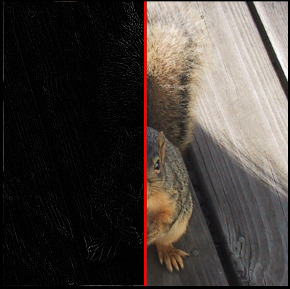
giving these increasingly blurry images
less blurry frog

Convolution

Filtering an image using a convolution kernel. This will lead nicely into the GPGPU work coming soon.

Some issues:

- We have seen that each fragment is processed independently (and perhaps in parallel) so how does the fragment shader get access to data from its neighbourhood? We have been passing a texture coordinate to the fragment shader. Now we will also need to let the fragment shader know the dimensions of the texture. Given the dimensions of the texture (e.g. 512 x 512) the fragment shader can calculate the texture coordinates of the neighbours and do additional texture lookups.

- We also don't have 2-dimensional arrays so we need to use 1-dimensional arrays for the kernel, indexed appropriately.

- We can make the kernel any size we want, though performance will be affected by larger kernel sizes.

There are examples on web link given next, which also illustrates some of the issues in using GLSL on different graphics cards with different capabilities:

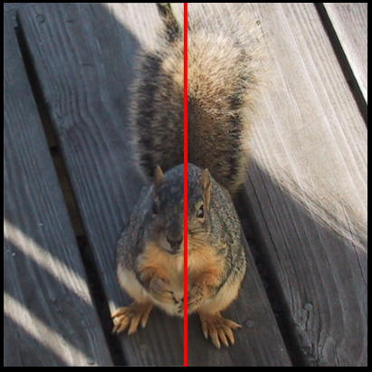
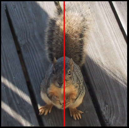
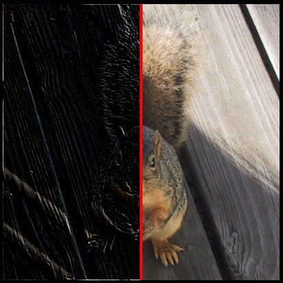
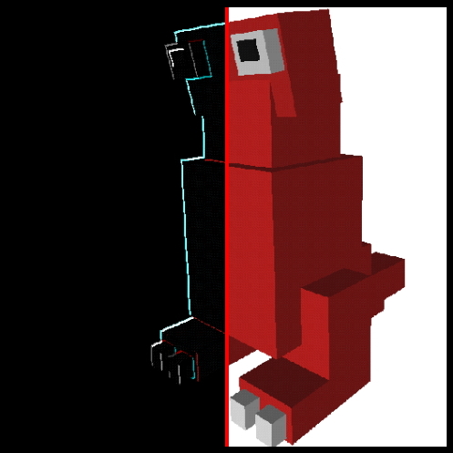
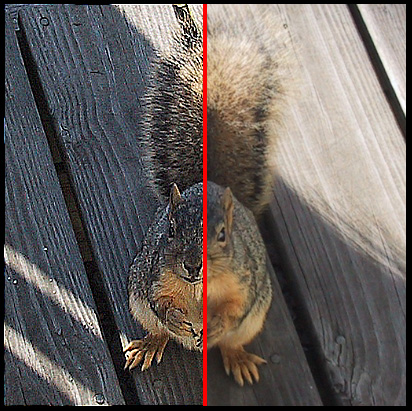
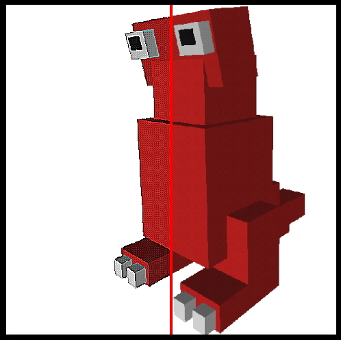
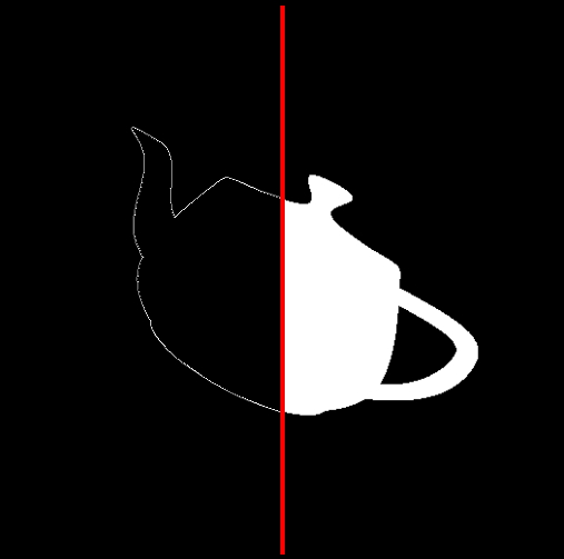
http://www.ozone3d.net/tutorials/image_filtering.php

I tried to create my own hybrid of the various code given there that would be pretty generic. This shader is nice because it splits the image in half and shows does the convolution only on the left-hand side.

Vertex Shader (same as before)

varying vec2 TexCoord;

void main (void)
{
    TexCoord = gl_MultiTexCoord0;
    gl_Position = ftransform();

}

Fragment Shader

#define KERNEL_SIZE 9

// Gaussian kernel
varying vec2 TexCoord;
float kernel[KERNEL_SIZE];

uniform sampler2D colorMap;
float width = 512.0;
float height = 512.0;

float step_w = 1.0/width;
float step_h = 1.0/height;

vec2 offset[KERNEL_SIZE];

void main(void)
{
   vec4 sum = vec4(0.0);

   offset[0] = vec2(-step_w, -step_h);
   offset[1] = vec2(0.0, -step_h);
   offset[2] = vec2(step_w, -step_h);

   offset[3] = vec2(-step_w, 0.0);
   offset[4] = vec2(0.0, 0.0);
   offset[5] = vec2(step_w, 0.0);

   offset[6] = vec2(-step_w, step_h);
   offset[7] = vec2(0.0, step_h);
   offset[8] = vec2(step_w, step_h);

   kernel[0] = 1.0/16.0; kernel[1] = 2.0/16.0;  kernel[2] = 1.0/16.0;
   kernel[3] = 2.0/16.0;  kernel[4] = 4.0/16.0; kernel[5] = 2.0/16.0;
   kernel[6] = 1.0/16.0;  kernel[7] = 2.0/16.0; kernel[8] = 1.0/16.0;


   if(TexCoord.s<0.495) // left of the center line - use convolution
       {

   
vec4
tmp
=
texture2D(colorMap,
TexCoord.st
+
      offset[0]);

          sum += tmp *
      kernel[0];

          tmp =
      texture2D(colorMap, TexCoord.st + offset[1]);

          sum += tmp *
      kernel[1];

          tmp =
      texture2D(colorMap, TexCoord.st + offset[2]);

          sum += tmp *
      kernel[2];

          tmp =
      texture2D(colorMap, TexCoord.st + offset[3]);

          sum += tmp *
      kernel[3];

          tmp =
      texture2D(colorMap, TexCoord.st + offset[4]);

          sum += tmp *
      kernel[4];

          tmp =
      texture2D(colorMap, TexCoord.st + offset[5]);

          sum += tmp *
      kernel[5];

          tmp =
      texture2D(colorMap, TexCoord.st + offset[6]);

          sum += tmp *
      kernel[6];

          tmp =
      texture2D(colorMap, TexCoord.st + offset[7]);

          sum += tmp *
      kernel[7];

          tmp =
      texture2D(colorMap, TexCoord.st + offset[8]);

          sum += tmp *
      kernel[8];

        } // right of the center line - leave the image alone
   else if( TexCoord.s>0.505 )
       {
        sum = texture2D(colorMap, TexCoord.xy);
       }
   else // on the center line - draw red
       {
        sum = vec4(1.0, 0.0, 0.0, 1.0);
       }

   gl_FragColor = sum;
}

We will be using these images as the sources:

normal squirrel

The code above uses a gaussian filter to blur the image
// 1/16 2/16 1/16
// 2/16 4/16 2/16
// 1/16 2/16 1/16

blurry squirrel

Mean filter to reduce noise
// 1/9 1/9 1/9
// 1/9 1/9 1/9
// 1/9 1/9 1/9

mean squirrel

Laplace Transform for edge detection
// 0 1 0
// 1 -4 1
// 0 1 0

edge enhanced
squirrel

Embossing
// 2 0 0
// 0 -1 0
// 0 0 -1

embossed squirrel

Shapening
// -1 -1 -1
// -1 9 -1
// -1 -1 -1

sharp squirrl

In all those cases we started with a texture and then manipulated it. Another approach is to use OpenGL (possibly with some shaders) to generate some 3D graphics, capture the 2D image of those graphics, then use that as a texture for another pass through a different set of shaders.

Once you have done the first pass and rendered some graphics, you copy the contents of the frame buffer back into a texture:

   glBindTexture(GL_TEXTURE_2D, frame);
   glCopyTexSubImage2D(GL_TEXTURE_2D, 0, 0, 0, 0, 0, winWidth, winHeight);

Read the texture data back out of the texture
    glGetTexImage(GL_TEXTURE_2D, 0, GL_RGB, GL_UNSIGNED_BYTE, frameBuf);

Flip it upside down so its rightside up
    for (h=0; h<winHeight;h++)
        memcpy(&frameBufFlip[end-h*rowSize], &frameBuf[h*rowSize], rowSize);

and then store the now rightside up texture for use with the convolution kernels
    glBindTexture(GL_TEXTURE_2D, frameFlip);
    glTexImage2D(GL_TEXTURE_2D, 0, GL_RGB, 512, 512, 0, GL_RGB,
        GL_UNSIGNED_BYTE, (const GLvoid *) frameBufFlip);

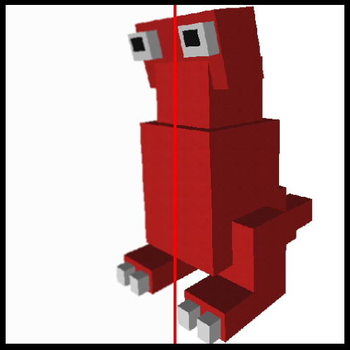
So I could draw the typical teapot and dynamically turn it around and then run the resulting image through the convolution kernels above to get this outline of a teapot. Quite a few graphical shader effects require multiple passes.

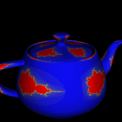
and here is a gzipped tar file of the convolution code

Mandelbrot

This code is pretty much straight out of the orange book. It is similar to the brick shader in that it procedurally generates a texture

vertex shader

// Vertex shader for drawing the Mandelbrot set
// Authors: Dave Baldwin, Steve Koren, Randi Rost
//          based on a shader by Michael Rivero
// Copyright (c) 2002-2004: 3Dlabs, Inc.
// See 3Dlabs-License.txt for license information
//

vec3 LightPosition = vec3(1.0, 1.0, 4.0);
float SpecularContribution = 0.1;
float DiffuseContribution = 0.9;
float Shininess = 0.2;

varying float LightIntensity;
varying vec3 Position;

void main(void)
{
    vec3 ecPosition = vec3 (gl_ModelViewMatrix * gl_Vertex);
    vec3 tnorm      = normalize(gl_NormalMatrix * gl_Normal);
    vec3 lightVec   = normalize(LightPosition - ecPosition);
    vec3 reflectVec = reflect(-lightVec, tnorm);
    vec3 viewVec    = normalize(-ecPosition);
    float spec      = max(dot(reflectVec, viewVec), 0.0);
    spec            = pow(spec, Shininess);
    LightIntensity = DiffuseContribution *
                          max(dot(lightVec, tnorm), 0.0) +
                          SpecularContribution * spec;
    Position        = vec3(gl_MultiTexCoord0 - 0.5) * 5.0;
    gl_Position     = ftransform();

}

Fragment Shader

// Fragment shader for drawing the Mandelbrot set
// Authors: Dave Baldwin, Steve Koren, Randi Rost
//          based on a shader by Michael Rivero
// Copyright (c) 2002-2004: 3Dlabs, Inc.
// See 3Dlabs-License.txt for license information
// tweaked a little bit by andy

varying vec3 Position;
varying float LightIntensity;

float MaxIterations = 120.0; // was 30.0 - how far can we zoom in
uniform float Zoom;
uniform float Xcenter;
uniform float Ycenter;
vec3 InnerColor = vec3(1.0, 0.0, 0.0); // red
vec3 OuterColor1 = vec3(0.0, 0.0, 1.0); // blue
vec3 OuterColor2 = vec3(1.0, 1.0, 0.0); // yellow

void main(void)
{
    float   real = Position.x * Zoom + Xcenter;
    float   imag = Position.y * Zoom + Ycenter;
    float   Creal = real;   // Change this line...
    float   Cimag = imag;   // ...and this one to get a Julia set

    float r2 = 0.0;
    float iter;

    for (iter = 0.0; iter < MaxIterations && r2 < 4.0; ++iter)
    {
        float tempreal = real;

        real = (tempreal * tempreal) - (imag * imag) + Creal;
        imag = 2.0 * tempreal * imag + Cimag;
        r2   = (real * real) + (imag * imag);
    }

    // Base the color on the number of iterations

    vec3 color;

    if (r2 < 4.0)
        color = InnerColor;
    else
        color = mix(OuterColor1, OuterColor2, fract(iter * 0.05));

    color *= LightIntensity;

    gl_FragColor = vec4 (color, 1.0);
}

allowing us to generate pretty pictures like the following
mandelbrot

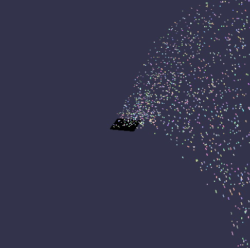
Particle System

Another example form the orange book. This confetti canon has a 2d array of particles (100 x 100) starting on a square. Each one has a random colour a random starting time, and a semi-random starting velocity. All of the 100x100 particles move through the vertex shader. Those that are 'alive' have their current position computed in the vertex shader (based on the current time, and their initial velocity) and are displayed as a point. The main application simply sets up the initial conditions and increments the time - the vertex shader handles all the computation. We will look at a similar particle system in cuda in a few weeks.

fragment shader:

varying vec4 Color;

void main (void)
{
    gl_FragColor = Color;
}

vertex shader:

uniform float Time;            // updated each frame by the application
uniform vec4 Background;      // constant color equal to background

attribute vec3 Velocity;      // initial velocity
attribute float StartTime;     // time at which particle is activated

varying vec4 Color;

void main(void)
{
    vec4 vert;
    float t = Time - StartTime;

    if (t >= 0.0)
    {
        vert    = gl_Vertex + vec4 (Velocity * t, 0.0);
        vert.y -= 4.9 * t * t;
        Color   = gl_Color;
    }
    else
    {
        vert = gl_Vertex;      // Initial position
        Color = Background;     // "pre-birth" color
    }

    gl_Position = gl_ModelViewProjectionMatrix * vert;
}

in the application:

static GLint arrayWidth, arrayHeight;
static GLfloat *verts      = NULL;
static GLfloat *colors = NULL;
static GLfloat *velocities = NULL;
static GLfloat *startTimes = NULL;

void createPoints(GLint w, GLint h) // 100 by 100 in the example
{
        GLfloat *vptr, *cptr, *velptr, *stptr;
        GLfloat i, j;

        if (verts != NULL)
            free(verts);

        verts      = malloc(w * h * 3 * sizeof(float));
        colors     = malloc(w * h * 3 * sizeof(float));
        velocities = malloc(w * h * 3 * sizeof(float));
        startTimes = malloc(w * h * sizeof(float));

        vptr   = verts;
        cptr = colors;
        velptr = velocities;
        stptr = startTimes;

        for (i = 0.5 / w - 0.5; i < 0.5; i = i + 1.0/w)
                for (j = 0.5 / h - 0.5; j < 0.5; j = j + 1.0/h)
                {
                        // starting location on the square
                        *vptr       = i;
                        *(vptr + 1) = 0.0;
                        *(vptr + 2) = j;
                        vptr += 3;

                        // colour tends to be bright (at least 0.5 for r, g, and b)
                        *cptr       = ((float) rand() / RAND_MAX) * 0.5 + 0.5;
                        *(cptr + 1) = ((float) rand() / RAND_MAX) * 0.5 + 0.5;
                        *(cptr + 2) = ((float) rand() / RAND_MAX) * 0.5 + 0.5;
                        cptr += 3;

                        // initial velocity has more y so the particle will go upwards more
                        *velptr       = (((float) rand() / RAND_MAX)) + 3.0;
                        *(velptr + 1) = ((float) rand() / RAND_MAX) * 10.0;
                        *(velptr + 2) = (((float) rand() / RAND_MAX)) + 3.0;
                        velptr += 3;

                        // random start time
                        *stptr = ((float) rand() / RAND_MAX) * 10.0;
                        stptr++;
                }

        arrayWidth = w;
        arrayHeight = h;
}

        glBindAttribLocation(ProgramObject, VELOCITY_ARRAY, "Velocity");
        glBindAttribLocation(ProgramObject, START_TIME_ARRAY, "StartTime");

void drawPoints() // each time trough the draw loop we do this
{
        glPointSize(2.0);

        glVertexPointer(3, GL_FLOAT, 0, verts);
        glColorPointer(3, GL_FLOAT, 0, colors);
        glVertexAttribPointer(VELOCITY_ARRAY, 3, GL_FLOAT, GL_FALSE, 0, velocities);
        glVertexAttribPointer(START_TIME_ARRAY, 1, GL_FLOAT, GL_FALSE, 0, startTimes);

        glEnableClientState(GL_VERTEX_ARRAY); // initial particle position
        glEnableClientState(GL_COLOR_ARRAY); // particle colour
        glEnableVertexAttribArray(VELOCITY_ARRAY);   // index 3 - initial velocity
        glEnableVertexAttribArray(START_TIME_ARRAY); // index 4 - starting time

        glDrawArrays(GL_POINTS, 0, arrayWidth * arrayHeight); // 100 by 100

        glDisableClientState(GL_VERTEX_ARRAY);
        glDisableClientState(GL_COLOR_ARRAY);
        glDisableVertexAttribArray(VELOCITY_ARRAY);
        glDisableVertexAttribArray(START_TIME_ARRAY);
}

     int location; // each time through the idle loop we do this

    location = getUniLoc(ProgramObject, "Time");
    ParticleTime += 0.002f;

    if (ParticleTime > 15.0)
    ParticleTime = 0.0;

    glUniform1f(location, ParticleTime);

When this course was taught in 2006 general computation on the GPU required the programmer to map the computational problem into a graphics problem. Nvidia's CUDA (Compute Unified Device Architecture) makes this easier by allowing a programmer to use C and familiar arrays to do work on the GPU.

http://www.nvidia.com/object/cuda_home_new.html

Rather than connecting multiple CPU cores together, or connecting multiple machines together into a compute cluster via MPI, CUDA gives a programmer access to a much large number of small parallel processors on a single card. While this capabilitity wont speed up your word processor, it can dramatically increase the speed of many computational applications. Aside from the practical speedups you can get from learning CUDA, programming for CUDA illustrates general techniques that are applicable to large scale parallel processing problems such as those that will be performed on NCSA's blue waters machine and other petascale computers.

CUDA works on Nvidia 8-series and newer cards. A list of supported cards is given here: http://www.nvidia.com/object/cuda_learn_products.html
eg the GeForce 8800 GTX has 128 thread processors can can have 12,288 active threads

a good CUDA introduction was given at SC 07: http://gpgpu.org/sc2007

and the current programming guide (4.1 as of November 2011): http://developer.download.nvidia.com/compute/DevZone/docs/html/C/doc/CUDA_C_Programming_Guide.pdf
gives a good introduction with more documentation at http://developer.nvidia.com/nvidia-gpu-computing-documentation

Some earlier related research projects included:

Brook Stream Programming Language on a GPU (requires an Nvidia card) http://graphics.stanford.edu/projects/brookgpu/index.html
Sh (for Windows, Linux, OS-X) http://libsh.org

and here are some code samples: http://developer.download.nvidia.com/compute/cuda/sdk/website/samples.html

Here is a simple example from supercomputing 07 comparing an array addition of two N by N matrices in the CPU and the GPU:

CPU C program fragment

void add_matrix_cpu (float *a, float *b, float *c, int N)
    {
    int i, j, index;
    for (i = 0; i < N; i++)
        {
        for ( j = 0 ; j < N; j++)
            {
            index = i + j*N;
            c[index] = a[index] + b[index];
            }
        }
}

void main()
    {
    add_matrix(a, b, c, N);
    }

CUDA C program fragment (assuming a single block so N < 24, a better version is given below)

__global__ void matAdd(float A[N][N], float B[N][N], float C[N][N])
    {
    int i = threadIdx.x;
    int j = threadIdx.y;

    if ( i < N && j < N)
        C[i][j] = A[i][j] + B[i][j];
    }

int main()
    {
    // Kernel invocation
    dim3 dimBlock(N, N);
    matAdd<<<1, dimBlock>>>(A, B, C);
    }

As with GLSL we split the problem solving into work in the main program on the CPU (or the host) and work that is done on the GPU. In graphics we have vertex shaders, geometry shaders, and fragment shaders, in CUDA we just have a single type of kernel.

In graphics whenever we pass vertices into the pipeline the currently active shaders are automatically run. In CUDA we specifically invoke the kernel when needed. Once invoked the GPU will deal with the kernel while the CPU will go on with its work (or wait if that's what you prefer).

A very important part of this is that you have to think about how to solve problems differently in this kind of computational environment. Instead of doing the computation in a specific order, each thread can run in parallel and each thread needs to know which part of the total problem it should work on so all the work gets done and the threads dont step over each other.

In the example above all of the threads have access to all three arrays. Each thread needs to work out which part of the arrays it is supposed to work with. In this case each thread finds its part of the array and handles one addition. Each thread could handle 1 addition, 3 additions, an entire row, etc depending on what is necessary. Its also possible (and likely) to have threads that start running but have no work to do.

CUDA has a lot of built-in flexibility on the assumption that there will be dramatic increases in the power of these 'graphics' cards. That means there are many ways to divide up and solve the same problem, and many different aspects that can be optimized for different hardware configurations.

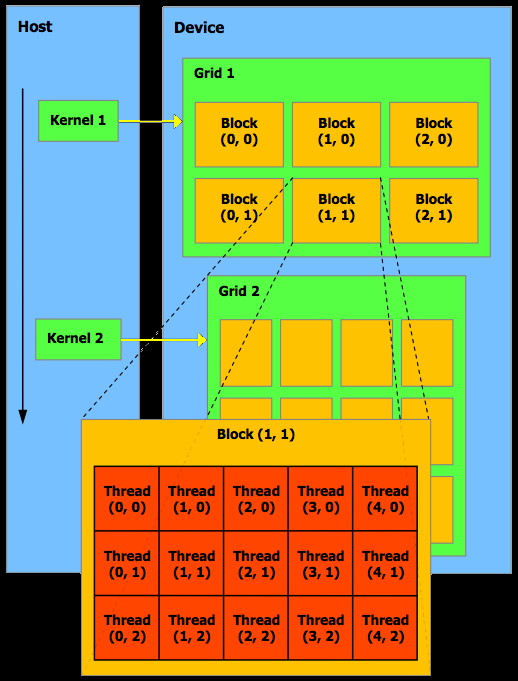
The programming guide goes into more detail about threads and blocks and grids.

A kernel can be executed by multiple equally-shaped thread blocks, so that the total number of threads is equal to the number of threads per block times the number of blocks. These multiple blocks are organized into a one-dimensional or two-dimensional grid of thread blocks. The dimension of the grid is specified by the first parameter of the <<<…>>> syntax. Each block within the grid can be identified by a one-dimensional or two-dimensional index accessible within the kernel through the built-in blockIdx variable. The dimension of the thread block is accessible within the kernel through the built-in blockDim variable.

For a one-dimensional block, the index of a thread and its thread ID are the same; for a 2D block of size (Dx, Dy), the thread ID of the thread with index (x, y) is (x + y Dx); for a 3D block of size (Dx, Dy, Dz), the thread ID of the thread with index (x, y, z) is (x + y Dx + z Dx Dy).

Threads within a block can cooperate among themselves by sharing data through some shared memory in the block and synchronizing their execution to coordinate memory accesses. More precisely, one can specify synchronization points in the kernel by calling the __syncthreads() intrinsic function; __syncthreads() acts as a barrier at which all threads in the block must wait before any are allowed to proceed. We will look at an example of this at the end of this page.

Here is a more general version of the code given above with a 2D grid of blocks and each block having a 2D (blocksize x blocksize) array of kernels:

__global__void add_matrix_gpu (float *a, float *b, float *c, int N)
    {
    int i = blockIdx.x * blockDim.x + threadIdx.x;
    int j = blockIdx.y * blockDim.y + threadIdx.y;
    int index = i + j*N;

    if ( i < N && j < N)
        c[index] = a[index] + b[index];
    }

void main()
    {
    dim3 dimBlock (blocksize, blocksize);
    dim3 dimGrid((N + dimBlock.x – 1) / dimBlock.x, (N + dimBlock.y – 1) / dimBlock.y);
    add_matrix_gpu <<< dimGrid, dimBlock>>> (a, b, c, N);
    }

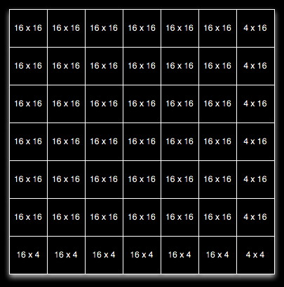
Lets say we set blocksize to 16 which gives us a maximum of 16 x 16 or 256 threads per block so blockDim.x and blockDim.y are each 16 and threadIdx.x and threadIdx.y each range from 0 to 15. Since we are adding 2D matrices we lay out the threads in the blocks and the blocks in the grid in a 2D array to make it easier to compute which matrix element each thread should work on, but that's just for convenience.

If N = 100 (i.e. we are adding two arrays that are 100 x 100 each) then dimGrid is 7,7 and blockIdx.x and blockIdx.y each range from 0 to 6.

This means that we have a 7 x 7 grid of blocks, each of which has 16 x 16 threads so 12,544 threads will be started to solve this problem for us, only 10,000 of which will do actual work.

Later on we will talk about how the arrays get into the memory of the graphics card.

With CUDA you have grids of blocks of threads.

Each thread has a thread ID. The threads within a block can be synchronized and have access to fast shared memory within the block as well as access to the slower global memory of the card. Threads in different blocks can not synchonize with each other. A block can contain a limited number of threads (currently 512). With CUDA threads can interact with each other - that was not true in the 'old' days of graphics-processing only GPUs.

A block has a block ID and can be specified as 1D, 2D, or 3D array of threads. Blocks of the same size and dimensionality are organized together into grids. Grids can be organized in 1D or 2D arrays. This is shown nicely in this image from the CUDA Programming Guide.

Each grid is handled by a single GPU. Each block (with a max of 512 threads) in the grid is handled by a single stream multiprocessor (could be anywhere from 1 to 120 stream multiprocessors) on that GPU. Each thread in the block is handled by a single stream processor within that stream multiprocessor. Each stream multiprocessor has 8 stream processors so # of multiprocessors * 8 gives you the number of cores on the GPU.

All of the blocks being processed at the same time are 'active' blocks. Registers and shared memory of a multiprocessor are split among the threads of the active blocks. Each active block is split into groups of threads called 'warps' where each warp contains the same number of threads - the 'warp size' (which is currently 32).

You can have a maximum of 8 active blocks per stream multiprocessor or a max of 24 active warps per stream multiprocessor. With 32 threads per warp that gives you a maximum of 768 active threads per stream multiprocessor. On a card like the GTX 285 that gives you 23,040 active threads. Note that you may not have enough other resources (registers, shared memory, etc) to perform the tasks efficiently, so its not just about having enough threads.

The Blocks and the warps within a block can execute in any order.

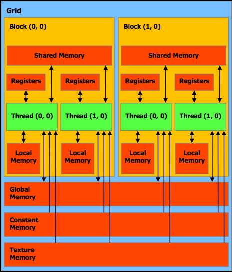
Each thread can:

Read-write	per-thread	registers	fastest
Read-write	per-thread	local memory	slow
Read-write	per-block	shared memory	fast
Read-write	per-grid	global memory	slow
Read-only	per-grid	constant memory	slow (but often cached)
Read-only	per-grid	texture memory	slow

This is shown nicely in this image from the CUDA Programming Guide.

Coming Next Time

Project 1 Presentations

last revision 1/29/2012