contains notes and images from:
Baraff, D., Rigit Body Simulation, An Introduction to Physically Based Modelling, SIGGRAPH 97 Course Notes.
http://particlesystems.elemeta.com/html/history.html
http://www.cs.wpi.edu/~matt/courses/cs563/talks/psys.html
We need the physics in the scene to be realistic enough to convey the concept. This usually means you can save time by not having to be completely realistic, but it can also mean that you may need to use 'wrong' physics if that generates the effect you want.
You need to match the visual style of the rest of the production. Some things will be physically modelled, others may be done with key-frame animation, or cell animation, or pencil drawings, or claymation, or muppets ... the CG should not look out of place (unless thats what you want)
Need to match the physics of the rest of the production. There is a certain type of physics that prevails in the Road Runner / Wile E. Coyote cartoons of Chuck Jones which is not the physics of the real world - e.g. any person running off the end of a cliff will stay suspended in the air for several seconds, any person falling large distances will make a hole 6 feet deep in the ground. Any physically based modelling done in that world should match the physics of that world.
Or you may want to reproduce real phenomena - the flying particles in the tornadoes in Twister, the waves of the hurricane in Perfect Storm.
You need the movements to be reproducible / controllable. The physically based elements will likely be combined with other elements so you cant just let those elements loose and 'see what happens.' The elements need to be choreographed, and once the choreography is correct it should be repeatable an infinite number of times.
Whats important is what ends up on the screen - what is visible to the audience. The audience won't know and shouldn't need to know how you did it. This allows you to cheat.
Here is a set of good introductions to various aspects of applying physics in games
with
more
information available here: http://www.d6.com/users/checker/dynamics.htm
When doing computer animation the animator usually has the luxury of not needing to work in real-time, so the physics can be more realistic, but we still want to get the job done within a realistic amount of time.
So
lets start
looking at particle systems - here we are going to look at particles
that go where they are told by the forces acting on them, but don't
interact with each other so each particle can be treated independently.
Particle systems will lead us into more complicated particle
interactions in physically-based modelling, and to living particles in
flocking.
Here
is where the math and the computer science come into things. The math
allows us to compute how the particles will move, and the computer
science allows us to optimize/parallelize/implement those calculations
and turn them into graphics. If this sort of thing was easy to animate
by hand then animators would do it by hand with traditional animation
or stop motion animation. For both the math and the computer science
there are simple algorithms that allow us to animate these particles in
a semi-realistic way. As more realism is needed the math gets more
complicated to do more accurate motion, and the algorithms get more
complicated to handle the particles more efficiently.
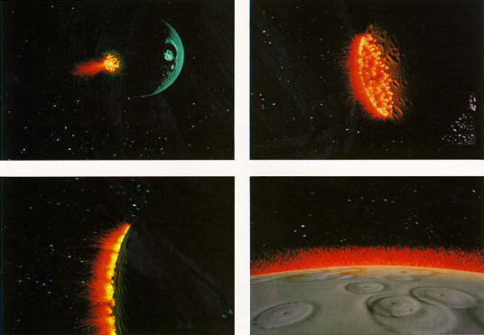
The term "particle system" was coined by William Reeves for his work in creating the "genesis effect" from Star Trek II: The Wrath of Khan
His
paper on it can be found here
He
needed to make
fire flow over the surface of this planetoid but didnt want the fire to
look like it was made of polygons. By using 'lots' of points as
particles he could give the computer graphics a 'fuzzy' stochastic
look.
His particles had the following properties:
Each of the particles go through three phases
Brief
look at the
Genesis Effect sequence from 1983.
and
a look at Karl Sims Particle Dreams at
http://www.archive.org/details/sims_particle_dreams_1988
and a few scenes from Twister - what a difference 15 years makes.
We have a bunch of particles. We need to know the position (and orientation and mass) of each particle to draw it in a given frame of the animation. We do not want to move each of the particles ourselves, but rather describe the forces that affect them (wind, gravity, an explosive force, all of the above, etc.) So we start with particles and forces. If we know the mass of the particle and the force applied to it then F=ma gives us the acceleration at any point in time. If we have an object rather than a point (and we ignore the rotation of the object) then we can pretend that the force acts on the center of mass of the object and treat it like a point.
Derivative
of
position is velocity: v= dx/dt
Derivative
of
velocity is acceleration: a=dv/dt
So we have a particle, and we know its mass and the forces acting on it at a particular instant of time, but what we need to know is where it will be at the time of the next animation frame. If the forces are constant then things are easy, but if the forces depend on the velocity or the position and we want to be realistic then that means we are need to integrate.
It
would be nice to
do analytical integration to go from acceleration to velocity and
position but usually thats too hard so we do numerical (approximate)
integration ...
which won't give us the exact answer but we can come close ... except
when it completely breaks down :)
The
trick is to find an appropriate step size that is small enough to be
realistic and not explode, but not so small that it takes too much time
to compute.
Euler - first order method - Given the current point use linear approximation to find the next point. Find the slope at the current point to get the tangent line. Go along the tangent line by the step size. Obviously a smaller step size (h or delta-t) leads to less error, but it also leads to more work. This method has an error of O(h2)
Xo initial value (position or velocity)
ti = t0 + h * i
d1
= f(ti,
Xi) so velocity is dependent on position and time,
acceleration on velocity and time
Xi+1 = Xi + h * d1
given
the velocity
at time i and the acceleration (sum of all forces / mass) at time i you
get the velocity at time i+1
given
position at
time i and velocity at time i you get the position at time i+1
Midpoint - second order method - Midpoint modifies Euler - instead of using the slope at the beginning of the time step, use the slope at the beginning to find the slope at the middle of the time step and use the slope at the middle to estimate the next position. It takes twice as much work, but this method has an error of O(h3)
Xo initial value (position or velocity)
d1
= f(ti,
Xi) // slope at the beginning of the interval
d2
= f(ti +
h/2, Xi
+ h/2 * d1) // slope at midpoint of interval using slope d1
Xi+1
= Xi
+ h * d2
Runge-Kutta -
fourth order method - like the midpoint version of the algorithm we
want to try and get closer to the actual slope to have a better
estimation. It takes 4 times as much work, but this method has an error
of O(h5) per step and acumulated error of O(h4)
Xo initial value (position or velocity)
d1
= f(ti,
Xi) // slope at the beginning of the interval
d2
= f(ti +
h/2, Xi
+ h/2 * d1) // slope at the midpoint using slope d1
d3
= f(ti +
h/2, Xi
+ h/2 * d2) // slope at the midpoint using slope d2
d4
= f(ti
+ h, Xi + h *
d3) // slope at the end of the interval
Xi+1
= Xi
+ h/6 *
(d1 + 2 * d2 + 2 * d3 + d4) // average with more weight at the middle
and
there is
the ever-useful wikipedia if you want more info:
http://en.wikipedia.org/wiki/Runge-Kutta
Particles
typedef
struct {
float m; // mass
float *x // position
float *v // velocity
float *f // force
acculumator
// and probably some other things that define other propoerties of the particle
}
*Particle
Forces
Unary forces - act on particles individually
n-ary forces - if n particles are connected by springs then all particles in that group will be affected
Spatial Interaction forces - attraction and repulsion may act on any/all pairs of particles depending on their positions
- gravitational attraction f = [G * ma * ma / (xa - xb)2 ] * (xa - xb) / || (xa - xb) || where G = 6.672 X 10⁻¹¹ Nm2kg-2
-
charge
(attraction / repulsion) f = k * |qa| |qb| / ||xa - xb||2 *
(xa - xb)
/ || (xa - xb) || where k = 8.9875 x 10⁹Nm2C-2
and here are some notes from the GPU programming course on doing these
sorts of things quickly on a GPU:
http://www.evl.uic.edu/aej/594/lecture06.html
Here is a nice particle system written in java
http://www.jhlabs.com/java/particles.html
There
are some nice
notes with diagrams at
http://www.cs.cmu.edu/~fp/courses/graphics/pdf-color/12-physical.pdf
Physically-based modelling