Project 2, CS 526: Allan Spale (aspale@evl.uic.edu)
Background
This program was written
using Python 2.1, VTK 4.2, and Tkinter (a Python module that supports GUI
widgets) and allows a user to visualize predefined datasets of the Visible
Woman. The files for the project are
simply project2.py. To run the program, type the following: python project2.py. Since Python is an interpreted language,
there is no need to compile; although there is an ability to compile a Python
script to decrease the startup time. The
program meets most of the basic requirements for displaying the requested
visualizations. Some additional
functionality was provided which will be described in the next section.
Sources
The sources of information
used to create this code include the following:
·
Python in a Nutshell, ISBN 0596001886 (used source as guideline to
construct GUI classes)
·
VTK Book,
ISBN 1930934076
·
Websites
o An
Introduction to Tkinter
o VTK Docs
o Python Docs
·
VTK Tk/Tcl
example code
·
Recommendations and
suggestions of other classmates
Usage
The GUI for this program is
a bit better than the first project.
However, there were some difficulties with getting stuff to appear as it
should. To simplify storing properties
for the VTK actors, the data was stored in the class used to create the dialog
windows. Because it was not as
straightforward as it seemed to make a fully functional modal dialog window and to keep the data persistent, the
dialog windows appear as soon as the program begins. They are accessible via the menu or the task
bar, but they may not be closed at any
time lest that dialog box not appear again.
An improvement over the last project was to increase the font size of
the widget objects in order to make them more readable. Unfortunately, this is counterbalanced with
some odd alignment with the label value that describes the value of the slider. Also related to the slider is that
fine-grained control regardless of the range of values is too-fined
grained. That is, each mouse click in
the non-button area of the slider click moves the slider a value of 1. However, moving the slider varies depending
on the range of values for that particular slider.
Generally, the program still
generally functions as one would expect without too many surprises. Using some combination of dataset and
visualization selections, it may be possible for the opacity function to stop
working and/or contours get a bit “noisy”.
For this reason, the author recommends going in menu order (head:
isosurface, raycast-composite, raycast-mip, feet: isosurface,
raycast-composite, raycast-MIP). This
may have been an anomaly that cannot be repeated, but for effective evaluation
of the visualizations, it is recommended that the user follows the above order.
To simplify matters, the
Female.raw file’s location was hard-coded to appear in the current directory
where the Python program resides. In
order to update the visualization, it is necessary to click in the rendering
window. It seemed fairly certain that a
recommendation from my classmate would have fixed the problem on how to code
this properly; unfortunately, this was not the case.
One other glaring problem
occurs with visualizing the feet dataset with raycasting. There is some odd clipping that occurs such
that the feet cannot be “zoomed into” directly.
For this reason, it is best to first visualize the feet using the
isosurface visualization, and then change to one of the raycast visualizations
of the feet. If the feet remain along
the edges when zooming in, this dataset will be better controlled. It seems that when a sampling rate is used
other than 1 (worked in the author’s test for 3, 3, 1), the clipping problem
seemed to subside somewhat.
By default, the joystick
control style (‘j’) is used to control the visualization. It can be turned off by pressing the ‘t’ key for
the trackball style of control.
There is no serious error
checking, but, fortunately, the GUI is presented in such a way as to strongly
eliminate any potential “syntax errors” but not logic errors (i.e. forgetting
that a surface was set to 0% opacity).
The menus are used in the
following manner:
Menus
·
Since the file
is “hard coded”, the only option here is to quit the program. To quit the program, either close the “main
window” (i.e. the one with the menu) or select Exit.
·
To visualize the
data, select two items from the two sections in the Visualization menu. The
available options for the first section are the visualization types which
include: Isosurface, Raycast-Composite, and Raycast-MIP (i.e. Maximum Instensity
Projection). The second section selecting
the dataset to view— Head or Feet.
Both of these also include a bit more of the body than there names would
literally imply. These menu selections
directly control what appears in the visualization, so no dialog window appears
for any of these menu selections. When
the program begins, isosurface is the default visualization and head is the
default dataset. More details about the
menu are as follows:
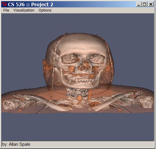
o Isosurfaces uses a marching cubes visualization to display predefined
single isovalue. In this case, bone is
determined to be a value of 860. Skin is
determined to be a value of 1250. This
visualization is the easiest to use to experiment with viewing the dataset.
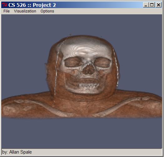
o Raycast-Composite uses a raycast composite function to visualize the
data. Because of poor performance by
selecting a single isovalue, ranges of isovalues are displayed for the skin and
bone isosurfaces. The actual range of
isosurfacfes displayed are very counterintuitive and were determined very much
by accident. Nonetheless, they seem to
present the best visualization that the author of the program could come up
with. The VTK Piecewise function used
for opacity displays a range of values 1250-5000 at increments of 10 for the
bone, and range of 860-1060 at increments of 5.
As determined by the author of this program, it is recommended to use an
opacity value of 100% for the bone and 5% for the skin. The VTK Color Transfer function was used for
the coloring of the isosurfaces. The
skin used a range of 860-960 at increments of 1, while the bone used a range of
1250-1509 at increments of 1. The bone
appears best when set to RGB value (255,255,255), while skin looks best as an
orange flesh-tone (in this author’s simple opinion and considering the fact no one
looks orange unless the individual has liver problems) with RGB value (255,140,81).
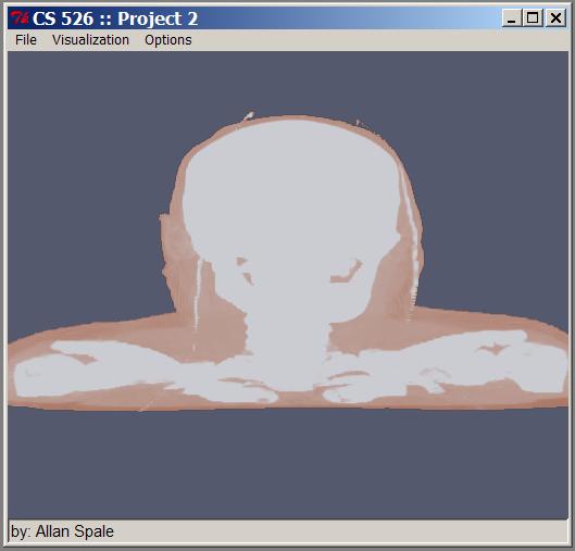
o Raycast-MIP uses a raycast maximum intensity projection function
to visualize the data. Again, because of
poor performance by selecting a single isovalue, ranges of isovalues are displayed
for the skin and bone isosurfaces. The
author was unable to get a suitable visualization for the bone that allows the
features of the bone to appear. Rather,
it appears more as a “solid silhouette” from all angles. The VTK Piecewise function used for opacity displays
a range of values 1250-5000 at increments of 1 for the bone, and range of 860-870
at increments of 1. As determined by the
author of this program, it is recommended to use an opacity value of 70% for
the bone and 50% for the skin. The VTK
Color Transfer function was used for the coloring of the isosurfaces. The skin used a range of 860-870 at
increments of 1, while the bone used a range of 1250-5000 at increments of 100. To keep colors similar to the other raycasting
visualization, the author recommends using an RGB value (255,255,255) for the
bone and an RGB value (255,140,81) for the skin.
o Head will display slices 0-100 from the entire dataset.
o Feet will display slices 500-576 from the entire
dataset.
·
To change some
of the options of how the dataset, select an item from the Options menu.
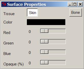
o Dataset
Properties allows the user to change
the RGB and opacity values a selected isosurface/tissue— bone or skin. As a benefit for the user, the current values
selected for red, green, and blue are blended together for the user to
see. Please note, when the user is done using this dialog box, it should be minimized and
not closed in order to avoid losing
the dialog window completely. Also
it is important to know that changes are
updated when the user clicks in the visualization portion of the main
window.
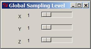
o Global Level
of Detail, allows the user to change
the sampling rate of the length (x-axis) and width (y-axis) of the slice in
addition to the number of slices (z-axis) used to define the model. The values for setting each of the axes range
from 1-8. Since the dimensions of the
entire dataset is 256x256x577, selecting a value results in dividing the
resolution for that axis by the value for the slider. These values can be set independently of one
another. To somewhat reduce the
unpleasantness of sampling, a polygon smoothing function is used by the render
to smooth the surfaces, regardless of what sampling values are used.
Design
There is a class that takes
care of all of the rendering. In the
constructor part of this class, all of the visualization pipeline parts are
created. Objects mapped to the renderer
are usually done in a way appropriate for the visualization. Below is the contruction of the pipelines:
readerVolume
[vtkImageReader]
|
+-- voiFeet [vtkExtractVOI]
| |
| +--
mapperCompFeet [vtkVolumeRayCastMapper]
| | |
| | +-- SetVolumeRayCastFunction
| | |
| | +-- compositeFunction [vtkVolumeRayCastCompositeFunction]
| |
| +--
mapperMIPFeet [vtkVolumeRayCastMapper]
| | |
| | +-- SetVolumeRayCastFunction
| | |
| | +-- compositeFunctionMIP [vtkVolumeRayCastCompositeFunction]
| |
| +-- contourBoneFeet
[vtkMarchingCubes]
| | |
| | +-- geoVolumeBone [vtkPVGeometryFilter]
| | |
| | +-- geoBoneMapper
[vtkPolyDataMapper]
| | |
| | +-- actorBone [vtkLODActor]
| |
| +-- contourSkinFeet
[vtkMarchingCubes]
| |
| +-- geoVolumeSkin [vtkPVGeometryFilter]
| |
| +-- geoSkinMapper
[vtkPolyDataMapper]
| |
| +-- actorSkin [vtkLODActor]
|
|
+-- voiHead [vtkExtractVOI]
| |
| +--
mapperCompHead [vtkVolumeRayCastMapper]
| | |
| | +-- SetVolumeRayCastFunction
| | |
| | +-- compositeFunction [vtkVolumeRayCastCompositeFunction]
| |
| +--
mapperMIPHead [vtkVolumeRayCastMapper]
| | |
| | +-- SetVolumeRayCastFunction
| | |
| | +-- compositeFunctionMIP [vtkVolumeRayCastCompositeFunction]
| |
| +-- contourBoneHead
[vtkMarchingCubes]
| | |
| | +-- geoVolumeBone [vtkPVGeometryFilter]
| | |
| | +-- geoBoneMapper
[vtkPolyDataMapper]
| | |
| | +-- actorBone [vtkLODActor]
| |
| +-- contourSkinTop
[vtkMarchingCubes]
| |
| +-- geoVolumeSkin [vtkPVGeometryFilter]
| |
| +-- geoSkinMapper
[vtkPolyDataMapper]
| |
| +-- actorSkin [vtkLODActor]
volumePropertyComp
[vtkVolumeProperty]
|
+-- SetScalarOpacity
| |
| +--
opacityFunctionComp [vtkPiecewiseFunction]
|
+-- SetColor
|
+-- colorTransferFunctionComp [vtkColorTransferFunction]
volumeComp
[vtkVolume]
|
+-- SetMapper
| |
| +--
mapperCompHead [vtkVolumeRayCastMapper]
| |
| +-- mapperCompFeet [vtkVolumeRayCastMapper]
|
+-- SetProperty
|
+-- volumePropertyComp [vtkVolumeProperty]
volumePropertyMIP
[vtkVolumeProperty]
|
+-- SetScalarOpacity
| |
| +--
opacityFunctionMIP [vtkPiecewiseFunction]
|
+-- SetColor
|
+-- colorTransferFunctionMIP [vtkColorTransferFunction]
volumeMIP
[vtkVolume]
|
+-- SetMapper
| |
| +--
mapperMIPHead [vtkVolumeRayCastMapper]
| |
| +-- mapperMIPFeet [vtkVolumeRayCastMapper]
|
+-- SetProperty
|
+-- volumePropertyMIP [vtkVolumeProperty]
Images
Please note,
the images taken here were before polygon smoothing was added to the program.
Opening
screenshot
Surface
properties dialog
Sampling
sizes dialog
All
images, unless otherwise noted, were taken at the original dataset resolution.
Isosurface
of head dataset
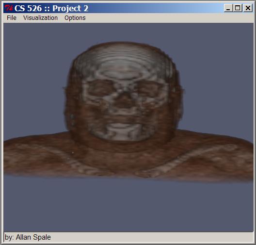
Raycasting
using a composite function on the head dataset
Raycasting
using a maximum intensity projection function on the head dataset
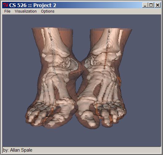
Isosurface
of feet dataset
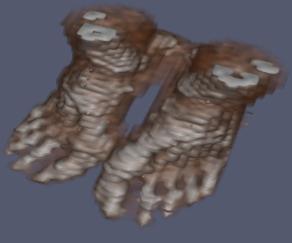
Raycasting
using a composite function on the feet dataset
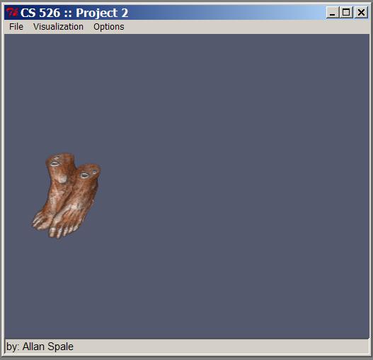
Because
of the clipping problem with the feet, here is an enlarged, somewhat
out-of-proportion enlargement of the same visualization.

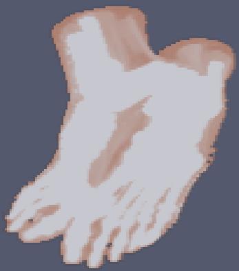
Raycasting
using a maximum intensity projection function on the feet dataset (enlarged and
not proportionate)
Sampling
of the dataset resolution is also possible.
In addition to dividing the resolution by the specified resolutions,
here is a ~ 85x85x1 of the head and feet: